ContentsFigures & Tables
With the accelerated electrification and intelligent transformation of the automotive industry, by-wire chassis systems have become a fundamental vehicle motion-control platform for new energy vehicles and autonomous driving [1, 2]. By replacing conventional mechanical or hydraulic transmission links with electronically controlled actuators, by-wire chassis systems provide higher control flexibility, faster response, and better integration with advanced vehicle dynamics control. Among different chassis subsystems, active suspension plays an important role in improving ride comfort, handling stability, and driving safety under complex road conditions [3–5]. Therefore, high-performance actuators with fast response, high reliability, and strong robustness are essential for the practical application of active suspension systems.
Electromagnetic linear actuators (EMLAs) are promising candidates for high-performance by-wire chassis actuation because they can directly convert electromagnetic energy into linear motion without intermediate motion conversion mechanisms. Compared with traditional servo motor drive systems, EMLAs significantly simplify the mechanical structure and offer advantages such as high efficiency, energy savings, compact structure, and fast dynamic response [6–8]. Owing to these benefits, EMLAs have been widely applied in automotive systems, precision manufacturing, aerospace engineering, and other high-precision actuation scenarios [9–11]. In automotive applications, active suspension systems require actuators capable of generating fast and controllable suspension forces to improve vibration suppression and ride comfort. In such suspension-oriented applications, large-stroke and high-force EMLAs are generally required. The EMLA investigated in this paper is a laboratory-scale EMLA system with a shorter stroke and lower force capacity than suspension-oriented EMLAs. Nevertheless, it shares the same electromagnetic force-generation mechanism, direct-drive characteristics, nonlinear dynamics, disturbance sensitivity, and actuator gain-fault features with suspension-oriented EMLAs. Therefore, it can serve as a representative platform for investigating fault diagnosis and fault-tolerant control methods for EMLA-based actuation systems.
However, the application of EMLAs in by-wire chassis and active suspension systems imposes stringent requirements on reliability and safety. During vehicle operation, suspension actuators are exposed to road disturbances, load variations, nonlinear friction, measurement noise, and possible actuator degradation. These factors may induce actuator gain faults, which change the effective input characteristics of the EMLA and deteriorate its overall actuation performance, control accuracy, and dynamic response. Moreover, due to the absence of intermediate transmission components, EMLAs are more sensitive to external disturbances and measurement noise. In practical applications, actuator gain faults may significantly degrade system performance, potentially leading to reduced control accuracy or even safety hazards [12]. Therefore, the development of effective fault diagnosis and fault-tolerant control (FTC) strategies for actuator gain faults is of great importance for ensuring the reliability and safety of EMLA systems.
In recent years, observer-based methods have been extensively investigated for fault diagnosis. Common approaches include Luenberger observers [13], unknown input observers [14], sliding mode observers [15], and iterative learning observers [16]. Among them, sliding mode observers exhibit strong robustness against disturbances, while iterative learning observers are effective in improving estimation accuracy by utilizing historical data. Several studies have attempted to combine these techniques to enhance fault estimation performance. For instance, iterative learning-based observers have been developed to estimate actuator faults under system uncertainties [17], while disturbance observers have been employed to achieve fault diagnosis using limited system information [18]. Chan et al. [19] developed a sliding mode observer tailored for nonlinear systems, which demonstrated robust fault estimation capabilities. Zhang et al. [20] proposed an integrated fault diagnosis framework that combines sliding mode observers with iterative learning unknown input observers, resulting in highly accurate fault estimation. Wang and Chi [21] introduced an iterative output observer that utilizes historical error data to estimate outputs under non-repetitive uncertainties, thereby enhancing tracking accuracy and robustness. Yang et al. [22] advanced the traditional high-gain disturbance observer by incorporating an iterative learning algorithm, which resulted in improved estimation accuracy for periodic disturbances. Wang et al. [23] developed an iterative learning observer capable of simultaneously estimating nonlinear terms and external disturbances, enhancing the observer's performance by integrating an adaptive algorithm. Despite these advances, existing methods still face challenges in achieving both high robustness and high estimation accuracy under complex operating conditions.
Regarding FTC strategies, active FTC methods have attracted considerable attention. Various approaches, such as adaptive control, sliding mode control, and multi-controller switching strategies, have been proposed to handle system faults [24, 25]. In particular, classified fault-tolerant control (CFTC) strategies, which apply different controllers according to fault severity, have shown promising performance improvements. Gong et al. [26] introduced an FTC approach utilizing multiple controllers by combining three types of FTC to achieve optimal FTC of the system. Xu et al. [27] combined hierarchical sliding mode control with neural network techniques to formulate an adaptive neural FTC scheme based on hierarchical sliding mode surfaces, thereby improving the fault tolerance of nonlinear systems. Wang et al. [28] presented an observer-based CFTC framework that utilizes different FTCs corresponding to varying fault severities, resulting in optimal FTC. However, research on integrating advanced observer-based fault diagnosis with CFTC strategies for EMLA systems remains relatively limited.
Motivated by the above observations, this paper proposes a novel fault diagnosis and CFTC scheme for EMLAs based on an improved sliding mode learning observer (ISMLO). The main contributions of this work are summarized as follows:
(i) A comprehensive mathematical model of the EMLA system is established by considering external disturbances, actuator gain faults, and measurement noise.
(ii) A proportional-derivative (PD)-type ISMLO with a forgetting factor is developed, which effectively enhances fault estimation accuracy and robustness against disturbances.
(iii) A CFTC strategy is designed based on fault estimation results, where different controllers are applied to minor and major faults to achieve improved overall fault-tolerant performance.
The remainder of this paper is organized as follows. Section 2 presents the mathematical modeling of the EMLA fault system. Section 3 describes the proposed ISMLO-based fault diagnosis method and provides the corresponding stability analysis. Section 4 develops the CFTC strategy and analyzes its stability. Section 5 validates the effectiveness of the proposed approach through hardware-in-the-loop experiments. Finally, Section 6 concludes the paper.
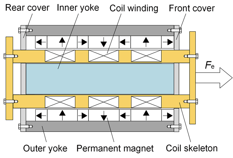
This paper considers a moving-coil EMLA based on a Halbach permanent magnet array. Although the considered EMLA differs from suspension-oriented EMLAs in structural parameters and operating conditions, it shares the same direct-drive electromagnetic actuation mechanism and similar nonlinear dynamic characteristics. Therefore, it can serve as a representative platform for investigating fault diagnosis and fault-tolerant control problems of EMLA-based actuation systems. The actuator consists of two main components: a mover and a stator. The mover includes the coil framework and the coil winding, while the stator is composed of permanent magnets, an outer yoke, and an inner yoke. The overall structure of the EMLA is illustrated in Figure 1, and detailed operating principles can be found in Reference [29].
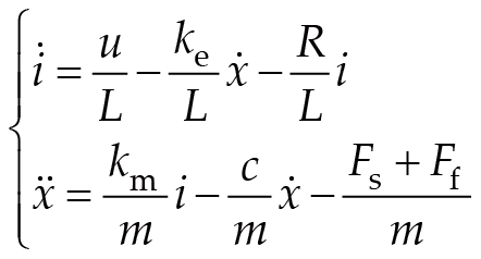
Based on electromagnetic and mechanical principles, the dynamic model of the EMLA can be expressed as:(1)where m is the mass of the mover, c is the damping coefficient, u and i are the power supply voltage and the current through the coil, respectively. R and L are the resistance and inductance of the entire coil, respectively. x, ẋ, and ẍ represent the position, velocity, and acceleration of the mover, respectively. km is the electromagnetic force constant, ke is the back electromotive force coefficient, with km and ke approximately equal. Fs is the external disturbance, and Ff is the nonlinear friction force.
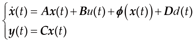
Define the state variable as , the input variable as u(t) = [u], the Lipschitz nonlinear term as ϕ(t) = [0 –Ff/m 0]T, and the external disturbance as d(t) = [Fs]. Then, the state-space representation of the EMLA system can be written as:(2)where , , , .
To facilitate subsequent analysis, the following assumptions are introduced.
Assumption (1): the nonlinear term ϕ(x(t)) is bounded, i.e., ‖ϕ(x(t))‖ ≤ ε, where ε is a positive constant.
Assumption (2): the nonlinear term ϕ(x(t)) satisfies the Lipschitz condition, i.e., , where γ is a positive Lipschitz constant.
Assumption (3): the external disturbance d(t) is bounded such that , where is a positive constant.
In practical applications, EMLAs may experience various types of faults [9], including actuator gain faults, bias faults, and sticking faults. Among these, gain faults—typically caused by magnetic leakage or actuator degradation—are one of the most common fault types. Therefore, this paper focuses on actuator gain faults.
When a gain fault occurs, the actual input of the actuator can be modeled as uf = (1−δ)u, where δ ∈ [0, 1] represents the gain loss coefficient. When δ = 0, the system operates normally; when 0 < δ < 1, a gain fault is present. The faulty input can be rewritten as Buf = Bu − Bδu = Bu + Ff(t). Considering external disturbances, actuator gain faults, and measurement noise, the state-space equations of the faulty EMLA system can be described by:(3)where F is the fault distribution matrix, E is the measurement noise distribution matrix, f(t) denotes the fault signal,η(t) represents measurement noise.
Assumption (4): the fault signal and measurement noise are bounded. The fault signal f(t) satisfies . In the mean square limit sense, the measurement noise η(t) and its derivative N(t) satisfy and , where , , and are all positive constants.
For subsequent stability analysis, the following lemmas are introduced.
Lemma (1): for any matrices X and Z with compatible dimensions, there exists a symmetric positive definite matrix H1 such that:(4)
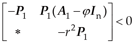
Lemma (2): for a given matrix A1∈Rn×n, there exists a symmetric positive definite matrix P1∈Rn×n such that:(5)where In denotes the n-dimensional identity matrix. In Equation (5), the eigenvalues of matrix A1 lie within a specified circular stability region D(φ, r), where the center and radius of the circular stability region are φ and r, respectively.
These assumptions and lemmas provide the theoretical foundation for the observer design and stability analysis presented in the subsequent sections.
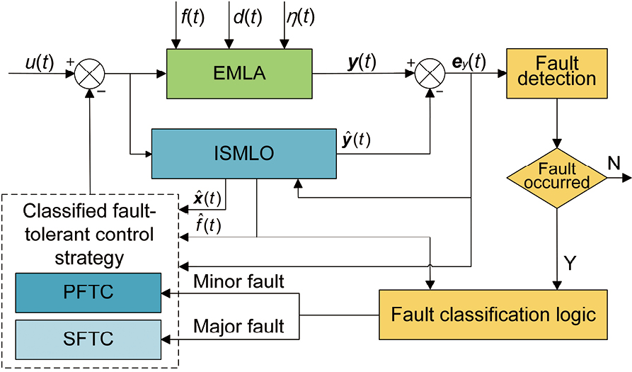
For the EMLA system in the presence of external disturbances, gain faults, and measurement noise, the overall framework of the fault diagnosis and CFTC scheme based on the ISMLO is illustrated in Figure 2. First, the ISMLO is designed to perform fault detection, state estimation, and fault estimation simultaneously. Once a fault is detected through the residual evaluation mechanism, the observer can rapidly track the system states and accurately estimate the fault. Based on the obtained fault estimation information, a CFTC strategy is subsequently constructed. According to the fault classification logic, faults are categorized into minor and major faults, for which the primary fault-tolerant control (PFTC) and secondary fault-tolerant control (SFTC) are employed, respectively. Finally, the control input is fed back to both the EMLA system and the ISMLO to compensate for faults, thereby ensuring stable operation of the system. This framework integrates fault diagnosis and control in a unified structure, improving both reliability and robustness.
To achieve accurate fault estimation and robust state estimation, a PD-type ISMLO is developed. The proposed observer combines the advantages of sliding mode control and iterative learning mechanisms, enabling strong robustness against disturbances and enhanced estimation accuracy. To improve estimation performance, a PD-type learning mechanism with a forgetting factor is introduced for fault estimation.
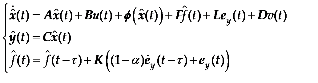
Define the output estimation residual as ey(t) = y(t)–ŷ(t). Based on Equation (3), the ISMLO is constructed as:(6)where is the estimated value of x(t), ŷ(t) is the estimated value of y(t), is the estimation of the nonlinear term, is the fault estimate value, L and K denote the observer gain matrices that require design, v(t) is the sliding mode control term, τ is the iterative learning interval, and α is the forgetting factor. The fault estimation law incorporates a PD-type iterative learning mechanism with a forgetting factor α, which improves convergence speed while preventing error accumulation.
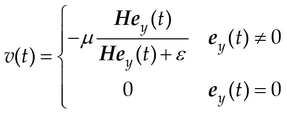
Let ey(t) be the sliding surface, the sliding mode control law is designed as follows:(7)where ε denotes a scalar constant with a very small value, H represents the gain matrix that requires design, and μ denotes the gain parameter to be designed.
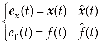
Define the state estimation error ex(t) and fault estimation error ef(t) as:(8)
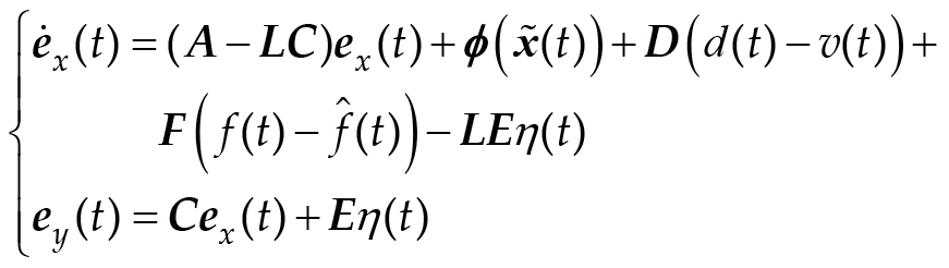
Integrating Equation (3) with Equation (6), the error equations can be derived as:(9)where , satisfies the Lipschitz condition, and .
Assumption (5): the fault matrix satisfies , where , and is a positive constant.
The following theorem is presented to establish sufficient conditions for the ultimate boundedness of the observer estimation errors and the corresponding H∞ performance of the estimation error system.
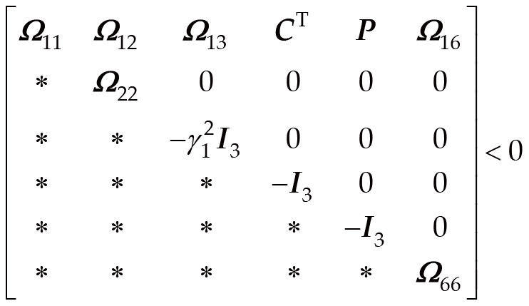
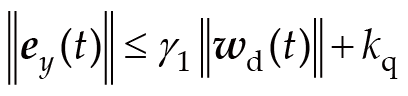
Theorem (1): consider the faulty EMLA system and ISMLO under Assumptions (1−5), if there exist positive definite matrices P∈R3×3 and Q∈R3×3, a matrix Y∈R3×3, matrices H∈R1×3 and K∈R1×3, as well as positive scalars γ and γ1, then by applying Lyapunov stability theory, Young's inequality, and bounding techniques for time-delay terms, the following linear matrix inequalities (LMIs) and equality constraints are derived:(10)(11)(12)(13)(14)where Ω11 = ATP + PA − YC − CTYT + Q + γ2I3, Ω12 = − PFKE − YE + CTE, Ω13 = − (1 − α)PFKE, Ω16 = PFKC, Ω22 = − γ12I + ETE, Ω66 = − I3/2(1 − α), Y = PL. Equations (12–14) are introduced to eliminate bilinear terms. If Equations (10–14) are satisfied, then ex(t) and ef(t) ultimately stabilize within a certain interval, and ey(t) satisfies:(15)where wd(t) = [ηT(t) NT(t)]T, kq is a positive constant.
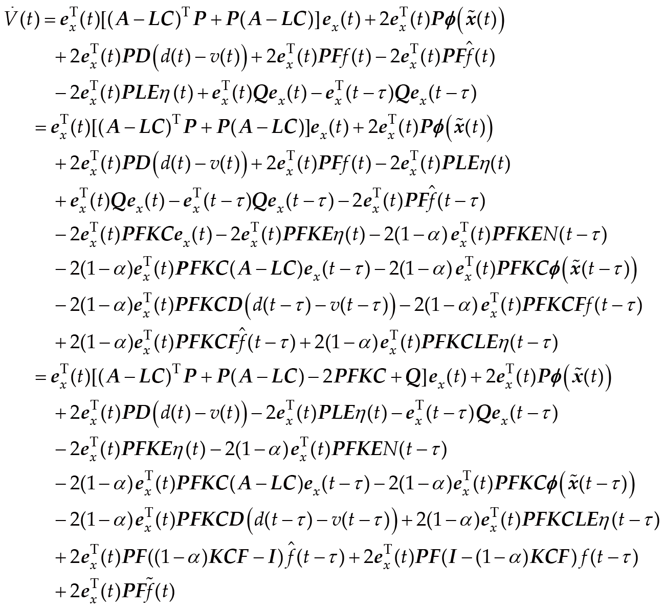
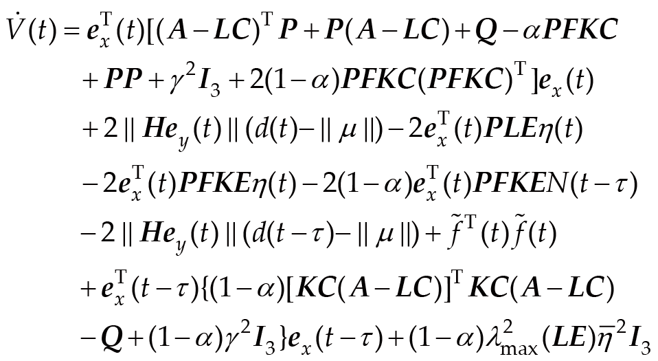
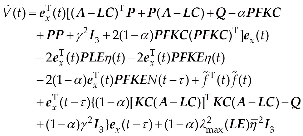
Proof: to analyze the stability of the error system, consider the following Lyapunov function:(16)which incorporates both instantaneous and historical information of the estimation error. The integral term captures the effect of the iterative learning interval, which is essential for ISMLO. Taking the derivative of the Lyapunov function yields:(17)
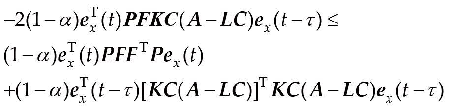
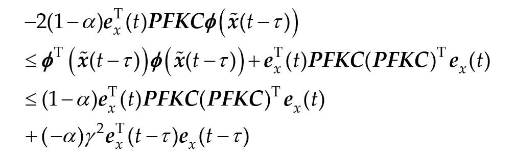
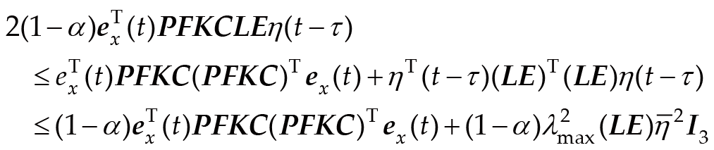
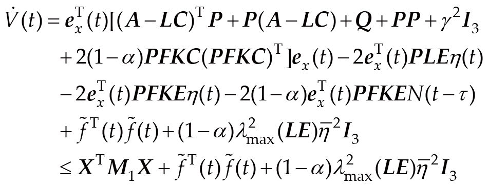
Based on Lemma (1) and Assumptions (1−5), the subsequent inequality is satisfied:(18)(19)(20)(21)(22)where λmax is the largest eigenvalue of matrix L. If Equations (12–14) are satisfied, substituting Equations (18–22) into Equation (17) yields:(23)
In the design, let the gain μ > 0, and μ ≥ d(t), μ ≥ d(t−τ), then it follows that:(24)
If Equation (11) holds, then according to the Schur complement lemma, then it follows that:(25)
If the forgetting factor α ≥ 0, then –αPFKC ≤ 0, and the following inequalities hold:(26)where , Π =, and .
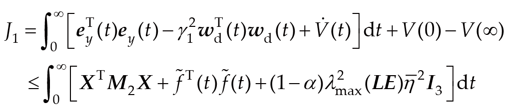
Define the H∞ performance index as:(27)
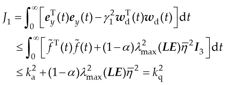
Under zero initial conditions, it can be obtained that:(28)where . If M2 < 0 holds true, then:(29)
where ka is a positive constant.
Therefore, if Assumptions (3–5) hold, then the H∞ performance index in Equation (15) is satisfied. If M2 < 0 holds, let Y = PL. Based on the Schur complement lemma, Equation (10) is satisfied. Proof completed.
It should be emphasized that Theorem (1) establishes the ultimate boundedness of the observer estimation errors, including ex(t) and ef(t), under bounded disturbances, measurement noise, and fault variations, rather than their asymptotic convergence to zero. Therefore, under practical operating conditions, the estimation errors ex(t) and ef(t) are generally not zero. These estimation errors should be treated as generally nonzero but ultimately bounded signals in the subsequent controller stability analysis rather than as signals that necessarily converge to zero.
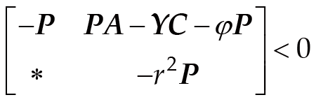
Note (1): to guarantee that the designed ISMLO exhibits robust convergence characteristics, the eigenvalues of matrix A−LC are placed within region (φ, r). As established in Lemma (2), the subsequent linear matrix inequality holds:(30)where r is a positive constant, φ is a negative constant, and |φ| ≥ r.
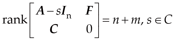
Note (2): regarding Theorem (1), a sufficient criterion ensuring the existence of an admissible solution for the proposed ISMLO is provided by:(31)where n = 3, m = 1, s is the complex frequency variable, and Equation (31) is equivalent to the condition that (A, F, C) possesses no invariant zeros located in the right half of the complex plane.
A residual fundamentally represents the difference between the actual output of a system and the output predicted by a corresponding model. Variations in the residual may indicate abnormal conditions or fault-related features within the system. In the context of fault detection, it is standard practice to develop a residual evaluation function and assess it against a predefined threshold to ascertain the presence of faults in the system.
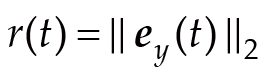
The residual evaluation function can be expressed as:(32)
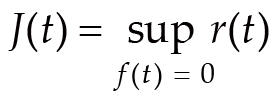
The preset threshold for the fault detectability index is denoted as:(33)
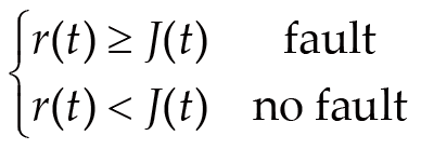
The fault detection logic can be expressed as:(34)
When r(t) exceeds the preset threshold J(t), it indicates that a fault has occurred in the EMLA. Otherwise, the EMLA is considered to be operating normally.
The objective of the control design is to ensure accurate trajectory tracking of the EMLA system in the presence of actuator gain faults, external disturbances, and measurement noise. Specifically, the controller should guarantee:
(i) The tracking error converges to a small neighborhood of zero;
(ii) The closed-loop system remains stable under both minor and major faults;
(iii) The control strategy adapts to different fault severities to improve overall performance.
To achieve these goals, a CFTC strategy for faults of varying severity is developed based on the fault estimation results provided by the ISMLO, which includes both PFTC and SFTC. The PFTC is developed utilizing ISMLO and state feedback to manage minor faults, while the SFTC is formulated utilizing state feedback and system output residuals to effectively mitigate major faults.
The SFTC, which incorporates system output residuals, performs better in fault tolerance when handling major faults. Therefore, the SFTC is employed in the occurrence of major faults. However, for systems experiencing minor faults, introducing system output residuals actually degrades fault-tolerant performance. Thus, the PFTC, which has better fault tolerance in such cases, is used when minor faults occur.
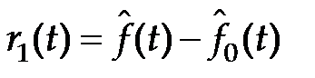
When EMLA experiences gain faults, the fault estimate value of ISMLO is , and the fault estimate value during normal system operation is defined as = 0.
The residual evaluation function may be formulated as:(35)
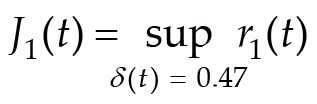
The preset fault classification threshold is defined as:(36)
The fault classification logic can be articulated as:(37)
When r1(t) remains below the preset threshold J1(t), this signifies a minor fault, prompting the activation of the PFTC. Conversely, if r1(t) surpasses the preset threshold J1(t), it indicates a major fault, thereby triggering the engagement of the SFTC.
This switching strategy ensures that:
(i) The PFTC is applied under minor fault conditions to maintain smooth control performance;
(ii) The SFTC is activated under major faults to enhance robustness and compensate for large uncertainties.
As a result, the proposed CFTC strategy achieves a balance between control performance and robustness under varying fault conditions.
Assumption (6): rang(B, F) = rank(B)
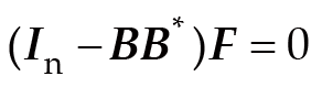
According to Reference [30], the above assumption is equivalent to the existence of a matrix B*∈ Rm×n, such that:(38)
The SFTC is designed as:(39)
Substituting Equation (39) into Equation (3) yields:(40)
Substituting Equation (38) into Equation (40) yields:(41)
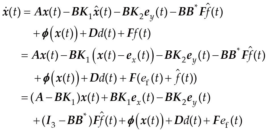
The secondary fault-tolerant controller uses the estimated states and estimated faults provided by the ISMLO. Therefore, the observer estimation errors enter the closed-loop dynamics. In the following controller stability analysis, the state estimation error ex(t), the fault estimation error ef(t), and the external disturbance d(t) are grouped into the lumped exogenous signal . According to Theorem (1), the observer estimation errors are ultimately bounded under bounded disturbances, measurement noise, and fault variations. Therefore, ex(t) and ef(t) are treated as exogenous components of ω(t) in the controller stability analysis rather than as signals that necessarily converge to zero.
The case ω(t) = 0 corresponds to an ideal unforced nominal reference case, where the observer estimation errors and external disturbances are absent, i.e., ex(t) = 0, ef(t) = 0, and d(t) = 0. In practical Hardware-in-the-Loop (HIL) tests or actual operation, the exact case ω(t) = 0 generally does not occur because disturbances, measurement noise, nonlinear effects, and observer estimation errors are present. Therefore, this case is not regarded as a practical operating condition. It is retained only as an ideal zero-input counterpart of the closed-loop system for examining the internal stability of the controller dynamics. For the practical case with ω(t) ≠ 0, asymptotic stability is not claimed; instead, the prescribed H∞ disturbance attenuation performance with respect to the lumped exogenous signal ω(t) is analyzed in the standard L2-gain sense.
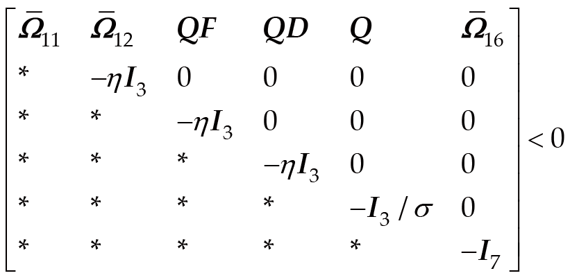
Theorem (2): For given scalars η > 0, σ > 0, and ρ > 0, if there exist a positive definite matrix Q ∈ R3×3 and matrices M ∈ R3×3 and N ∈ R3×3 that satisfy the H∞ performance index ‖x‖22 < η2‖ω‖22, and the following conditions are met, then the ideal unforced closed-loop system Equation (41) with ω(t) = 0 is asymptotically stable. When ω(t) ≠ 0, asymptotic stability is not claimed; instead, the closed-loop system satisfies the prescribed H∞ disturbance attenuation performance with respect to the lumped exogenous signal ω(t) in the L2-gain sense.(42)where , , .
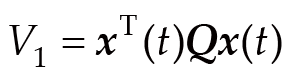
Proof: define the Lyapunov function as:(43)
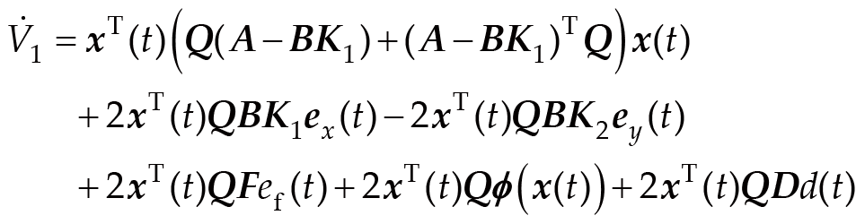
Taking the derivative of the Lyapunov function, then it follows that:(44)
Based on Young's inequality and Assumption (1), then it follows that:(45)
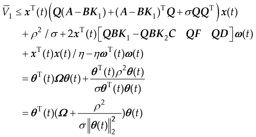
Substituting Equation (45) into Equation (44) and rearranging yields:(46)where .
Define , then it follows that:(47)where θ(t) = [xT(t) ωT(t)]T, , .
When ω(t) = 0, the closed-loop system corresponds to an ideal unforced nominal reference case, in which ex(t) = 0, ef(t) = 0, and d(t) = 0. If , namely, the matrix term is negative definite, then the derivative of the Lyapunov function satisfies for any nonzero state trajectory. Since V(t) is positive definite and is negative definite, the state of the ideal unforced closed-loop system converges asymptotically to the equilibrium point. Therefore, according to the Lyapunov stability theorem, the ideal unforced closed-loop system (Equation (41)) with ω(t) = 0 is asymptotically stable. By setting M = QBK1 and N = QBK2, and applying the Schur complement lemma, the above negative-definiteness condition can be transformed into the LMI condition Equation (42).
When ω(t) ≠ 0, the observer estimation errors and external disturbance are regarded as the lumped exogenous input to the closed-loop system. In this case, asymptotic stability is not claimed. Instead, the H∞ performance is considered in the L2-gain sense. From , the following performance index can be obtained under zero initial conditions:(48)
Thus, . That is, . Therefore, the closed-loop system satisfies the prescribed H∞ disturbance attenuation performance with respect to ω(t). The scalar η is selected such that the LMI condition Equation (42) is feasible. This result establishes the prescribed H∞ disturbance attenuation performance under nonzero ω(t), rather than asymptotic stability under nonzero disturbances or nonzero observer estimation errors. Proof completed.
Note (3): matrix B is a full column rank matrix, so its left inverse matrix B+ exists and is unique. According to Reference [31], B* = B+ and B+ = (BTB)−1BT, which further implies that K1 = B+Q−1M and K2 = B+Q−1N.
The PFTC is designed as:(49)
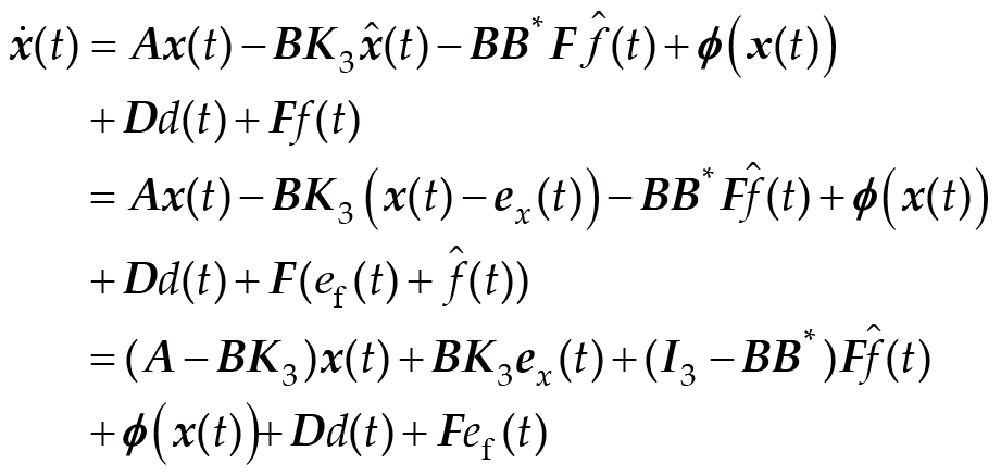
Substituting Equation (49) into Equation (3) yields:(50)
Substituting Equation (38) into Equation (50) yields:(51)
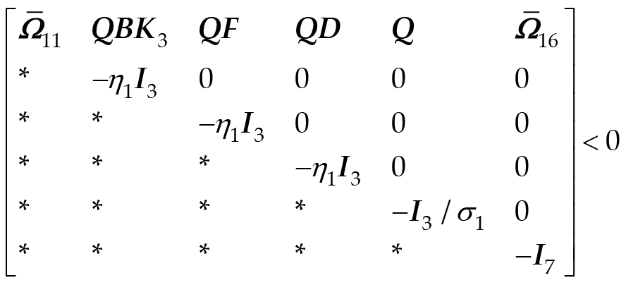
Theorem (3): for given scalars η1 > 0, σ1 > 0, and ρ1 > 0, if there exist a positive definite matrix Q ∈ R3×3 and a matrix K3 ∈ R1×3 that satisfy the H∞ performance index ‖x‖22 < η12‖ω‖22, and the following conditions are met, then the ideal unforced closed-loop system Equation (51) with ω(t) = 0 is asymptotically stable. When ω(t) ≠ 0, asymptotic stability is not claimed; instead, the closed-loop system satisfies the prescribed H∞ disturbance attenuation performance with respect to the lumped exogenous signal ω(t) in the L2-gain sense.(52)where , .
Proof: the proof follows a line of reasoning similar to that of Theorem (2). For the closed-loop system Equation (51), the Lyapunov function is selected as V(t) = xT(t)Qx(t), where Q = QT>0. Taking the derivative of V(t) along the trajectory of Equation (51), and applying Young's inequality together with Assumption (1), the nonlinear term can be bounded. Then, the derivative of the Lyapunov function can be transformed into a quadratic form associated with the matrix inequality in Equation (52).
If the LMI condition Equation (52) holds, then by applying the Schur complement lemma, the corresponding quadratic form is negative definite. When ω(t) = 0, the system corresponds to the ideal unforced nominal reference case, in which ex(t) = 0, ef(t) = 0, and d(t) = 0. In this case, holds for any nonzero state trajectory. Since the Lyapunov function is positive definite and its derivative is negative definite, the ideal unforced closed-loop system (Equation (51)) with ω(t) = 0 is asymptotically stable according to the Lyapunov stability theorem.
When ω(t) ≠ 0, the same H∞ performance analysis as in Theorem (2) can be obtained in the L2-gain sense. Under zero initial conditions, the closed-loop system satisfies . The scalar η1 is selected such that the LMI condition Equation (52) is feasible. Thus, Theorem (3) guarantees internal asymptotic stability only for the ideal unforced closed-loop system with ω(t) = 0, while for the practical case with nonzero ω(t), it guarantees the prescribed H∞ disturbance attenuation performance with respect to the lumped exogenous signal ω(t) in the L2-gain sense. Asymptotic stability under nonzero disturbances or nonzero observer estimation errors is not claimed. Proof completed.
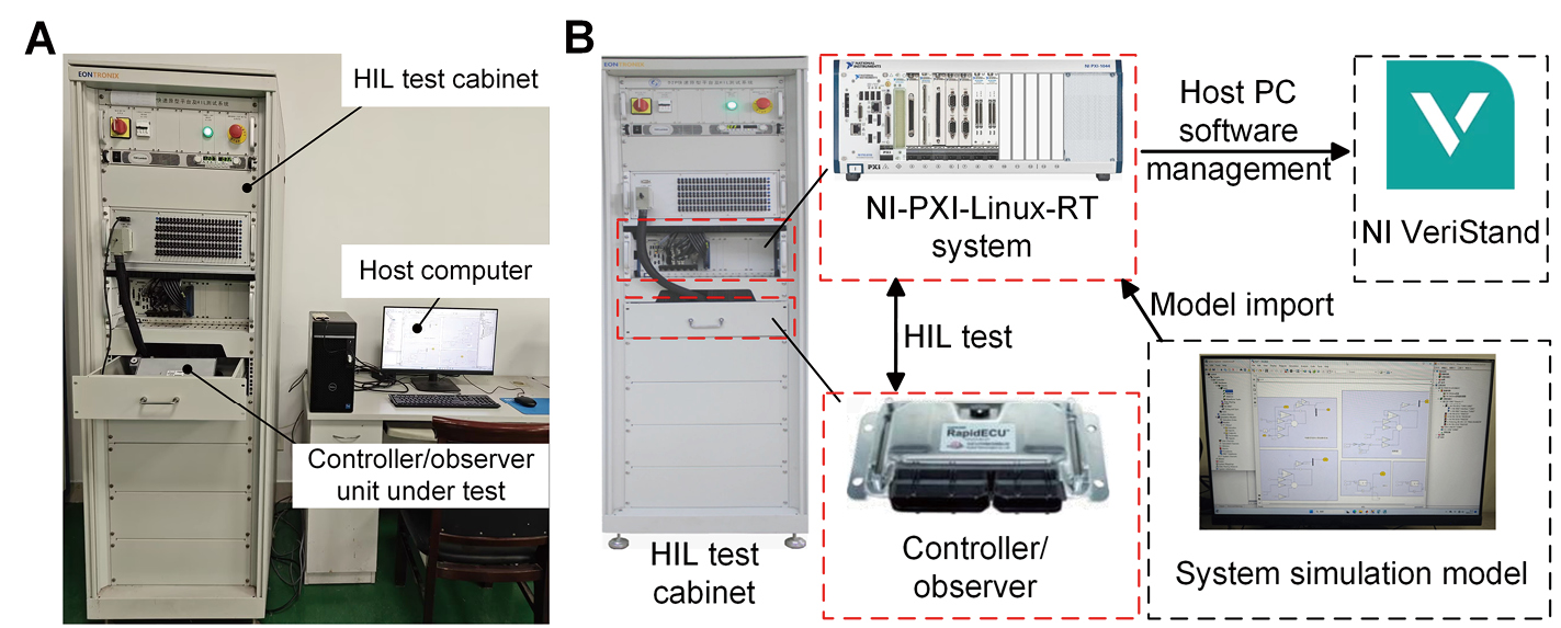
To validate the effectiveness of the proposed method, HIL experiments are conducted. HIL testing is a semi-physical simulation technology that can simulate the operating state of the object under test under laboratory conditions. The HIL test cabinet connects to the controller/observer under test through I/O interfaces. By integrating a real controller or using a real-time simulation model, it conducts comprehensive and systematic testing of the controller/observer under test. Using HIL testing for FTC offers significant advantages: it enables flexible fault injection, improves test safety, reduces development costs, and enhances the comprehensiveness and reliability of testing. Moreover, HIL testing provides a safe and repeatable environment for evaluating fault diagnosis and fault-tolerant control strategies under different fault conditions. Therefore, this paper utilizes the HIL test platform to validate the performance of the ISMLO and the CFTC strategy when the EMLA experiences faults.
Figure 3 shows the HIL test platform and the corresponding schematic diagram. It consists of the HIL test cabinet, a host computer, and the controller/observer under test. The NI-PXI-Linux-RT system (NI PXI, NI PXI-1044, Beijing Jiuzhou Huahai Technology Co., Ltd., Beijing, China) inside the HIL test cabinet connects to the controller/observer under test and is linked to the host computer via Ethernet. During testing, the control strategy is compiled into executable code and flashed onto the real controller. Meanwhile, the input and output ports of NI VeriStand Real-Time Testing Application Software (NI VeriStand, VeriStand 2018, National Instruments, Austin, Texas, USA) replace the corresponding ports in the system simulation model. Using the Linux system as the toolchain, the system simulation model is compiled into a dynamic library file, imported into the NI VeriStand software, deployed to the NI-PXI-Linux-RT system for execution, and the fault injection cards in the HIL test cabinet are used to implement various types and levels of fault injection. The test management software (NI VeriStand) on the host computer operates and manages the NI-PXI-Linux-RT system to complete the HIL testing.
The physical and electrical parameters of the EMLA are specified as follows: the mover mass m is 0.12 kg, the damping coefficient c is 5 Ns m−1, the coil resistance R is 1.41 Ω, the inductance L is 1.1 mH, the electromagnetic force coefficient km is 25 N A−1, the back electromotive force coefficient ke is 25 Vs m−1, and the actuator stroke is 10 mm. Before the EMLA experiences gain faults, a sinusoidal target displacement of 8 mm at a frequency of 4 Hz is applied. Measurement noise η(t) = 3 × 10⁻⁶ × sin(40 × pi × t), external disturbance d(t) = 0.2 × rand × sin(16 × pi × t), measurement noise matrix E = [1 1 0]T, fault matrix .
Although a sinusoidal target displacement is used in the HIL validation, the proposed ISMLO and CFTC scheme is not limited to sinusoidal reference trajectories. The observer and controller are designed based on the EMLA dynamic model, measured system signals, and closed-loop stability conditions, rather than the specific waveform of the reference trajectory. Therefore, the proposed method can be extended to other bounded reference trajectories, provided that the reference trajectory, system states, control input, disturbances, measurement noise, and fault variations remain bounded and the actuator physical constraints are satisfied.
The initial conditions for both the EMLA and the ISMLO are set to zero. When calculating the inequalities, parameters are defined as α = 0.4, γ = 0.01, γ1 = 2, φ = −10, τ = 10−4, μ = 3, η = 6.4 × 10⁴, σ = 1.4 × 10⁻⁵, η1 = 9 × 10⁴, and σ1 = 1 × 10⁻⁵. The parameter values for the conventional PD-type learning observer (LO) and the sliding mode observer (SMO) are the same as above. In addition, the proposed ISMLO, LO, and SMO are implemented under the same EMLA system parameters, initial conditions, target displacement, measurement noise, external disturbance, and fault injection conditions. Therefore, comparisons among different observers are conducted under the same operating, disturbance, and fault conditions to ensure a fair evaluation of their estimation performance.
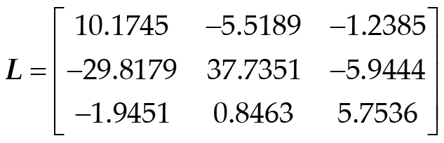
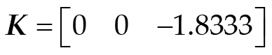
According to Theorem (1), using MATLAB's LMI toolbox to solve Equations (10–14), the observer gain matrices are obtained as follows:(53)(54)(55)
According to Theorems (2, 3), using MATLAB's LMI toolbox to solve Equations (42, 52), respectively, the FTC gain matrices are obtained as follows:(56)(57)(58)
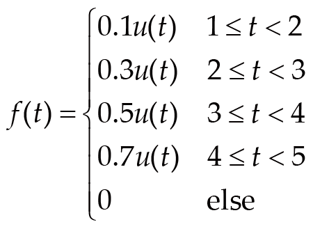
EMLA undergoes a 6-second HIL test with the following fault scenarios applied. The system operates under normal conditions from 0 to 1 s. A gain fault with δ = 0.1 is introduced from 1 to 2 s, followed by a gain fault with δ = 0.3 from 2 to 3 s. Subsequently, a gain fault with δ = 0.5 is imposed from 3 to 4 s, and a gain fault with δ = 0.7 is applied from 4 to 5 s. After 5 s, the system returns to the fault-free condition. The fault injection method is as follows:(59)
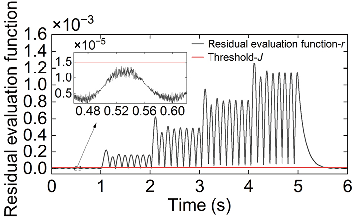
After gain faults occur in the EMLA, the fault detection performance of the ISMLO is illustrated in Figure 4. During the interval from 0 to 1 s, no gain fault is introduced. Due to external disturbances and measurement noise, the residual evaluation function does not remain strictly zero but fluctuates within the range of 2.1 × 10⁻⁶ to 1.4 × 10⁻⁵. This indicates that the sliding mode term incorporated in the ISMLO effectively suppresses disturbance-induced fluctuations, thereby maintaining a low residual level under healthy conditions. When gain faults are introduced in the interval from 1 to 5 s, the residual evaluation function exceeds the predefined threshold of 1.5 × 10⁻⁵. According to Equation (34), this indicates the occurrence of a fault. The clear separation between the fault-free and faulty residual levels demonstrates that the residual evaluation function is highly sensitive to gain faults while remaining robust to disturbances and measurement noise.
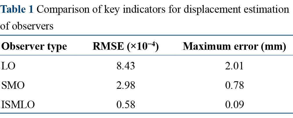
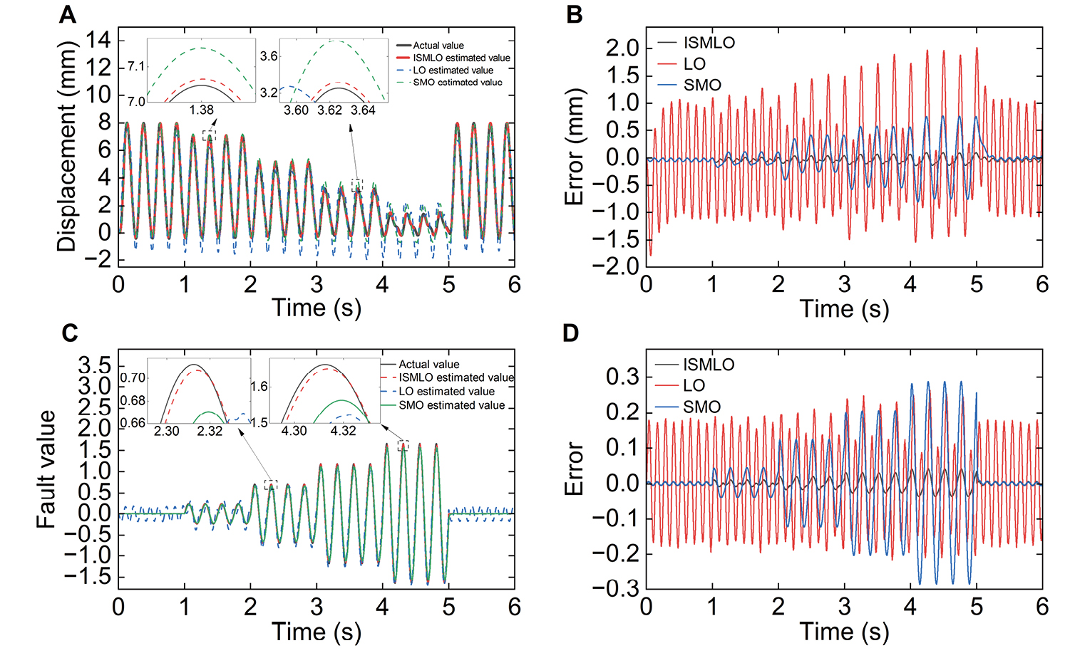
The proposed PD-type ISMLO is compared with a conventional PD-type LO and an SMO. The displacement estimation results are shown in Figure 5A, B, and the quantitative performance indicators are summarized in Table 1.
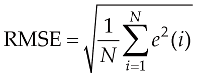
The root mean square error (RMSE) is calculated as:(60)where e(i) denotes the estimation error at the i-th sampling instant, and N is the total number of sampled data points. For displacement estimation, e(i) represents the difference between the actual displacement and the estimated displacement. For fault estimation, e(i) represents the difference between the actual fault value and the estimated fault value.
As shown in Figure 5A, B, under disturbance and measurement noise, the ISMLO tracks the actual displacement within 0.01 s at the initial stage. After the occurrence of gain faults, the observer maintains the same rapid convergence speed, demonstrating strong robustness and fast dynamic response. From Figure 5A, B and Table 1, the maximum displacement estimation error of the ISMLO is 0.09 mm, with a RMSE of 0.58 × 10⁻⁴. Compared with the LO and SMO, the proposed ISMLO reduces the maximum error by at least 88% and the RMSE by at least 80%. This improvement is mainly attributed to the combination of the sliding mode mechanism and the PD-type learning structure, which enhances disturbance rejection capability while preserving fast convergence. As a result, the ISMLO achieves high estimation accuracy and strong robustness, thereby improving fault estimation and FTC performance.
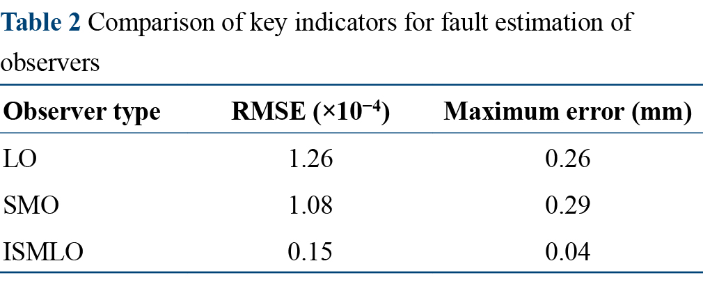
The fault estimation results are presented in Figure 5C, D, and the corresponding quantitative performance indicators are listed in Table 2. As shown in Figure 5C, D, the ISMLO achieves fault estimation within 0.003 s after the occurrence of a gain fault, indicating a very fast response speed. From Figure 5C, D and Table 2, the maximum fault estimation error is 0.04, with an RMSE of 0.15. Compared with the LO and SMO, the ISMLO reduces the maximum error by at least 86% and the RMSE by at least 86%. This superior performance demonstrates that the proposed observer provides highly accurate and robust fault estimation. The improved accuracy can be attributed to the learning mechanism with a forgetting factor, which effectively utilizes historical information while suppressing outdated data, thereby enhancing estimation performance under time-varying conditions.
The influence of the iterative learning interval τ on fault estimation performance is analyzed in Figure 6A, B. As observed in Figure 6A, a smaller iterative learning interval τ leads to improved fault estimation accuracy and reduced estimation error. This is because a shorter interval allows more frequent updates of the learning mechanism, resulting in faster error correction. The optimal interval selection process is illustrated in Figure 6B. When τ = 0.2, the peak absolute error (PAE) reaches 1.64. As τ decreases, the PAE decreases accordingly. When τ = 0.2, the PAE is reduced to 0.04, which satisfies the fault estimation requirements. Therefore, τ = 1 × 10⁻⁴ is selected as the optimal iterative learning interval, at which the ISMLO achieves the best estimation performance.
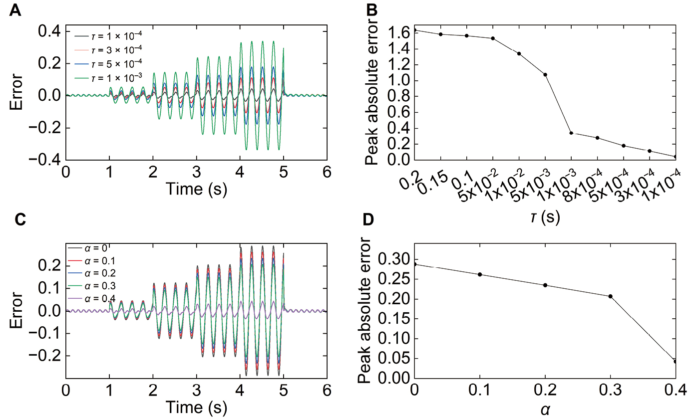
The influence of the forgetting factor α on fault estimation performance is analyzed in Figure 6C, D. As shown in Figure 6C, the estimation accuracy improves as α increases, and the best performance is achieved at α = 0.4. The optimal forgetting factor selection process is illustrated in Figure 6D. When α = 0, the PAE is 0.29. As α increases, the error decreases and reaches a minimum value of 0.04 at α = 0.4. When α exceeds 0.4, the observer matrix no longer satisfies the positive definiteness condition, indicating that the stability constraint limits the feasible range of α. Therefore, α = 0.4 is selected as the optimal forgetting factor, achieving the best trade-off between stability and estimation accuracy.
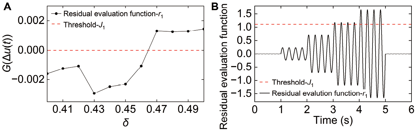
To determine the fault classification threshold J1(t), the fault-tolerant performance transition point δ is analyzed by comparing the control outputs of the SFTC and PFTC strategies. The control output difference is defined based on Equations (39, 49) as:(61)
Under the same fault condition, the performance evaluation index is defined as:(62)
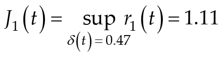
The fault-tolerant performance transition point δ is determined by evaluating G(Δu(t)) under different fault severities. The determination process of δ and the fault classification process are illustrated in Figure 7. As shown in Figure 7A, when the fault gain satisfies δ < 0.47, the performance index satisfies G(Δu(t)) < 0, indicating that the PFTC strategy provides superior control performance. In contrast, when δ ≥ 0.47, the performance index becomes G(Δu(t)) > 0, demonstrating that the SFTC strategy achieves better robustness and fault compensation capability under severe fault conditions. Therefore, the fault-tolerant performance transition point is determined as δ = 0.47, and the corresponding fault classification threshold is selected as:(63)Based on the proposed fault classification mechanism, when gain faults of δ < 0.47 occur, i.e., the residual evaluation function r1(t) does not exceed the preset threshold J1(t) = 1.11, PFTC is activated. When the gain faults of δ ≥ 0.47 occur, i.e., the residual evaluation function r1(t) exceeds the preset threshold J1(t) = 1.11, SFTC is activated. Based on the fault classification logic in Equation (37), the fault classification process is shown in Figure 7B. The results demonstrate that the proposed classification mechanism can effectively distinguish different fault severities and achieve reliable controller switching, thereby improving the robustness and fault-tolerant control performance.
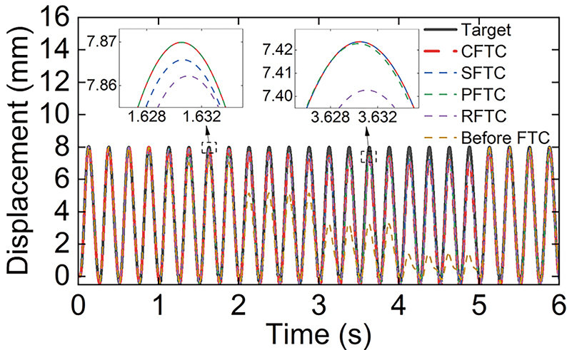
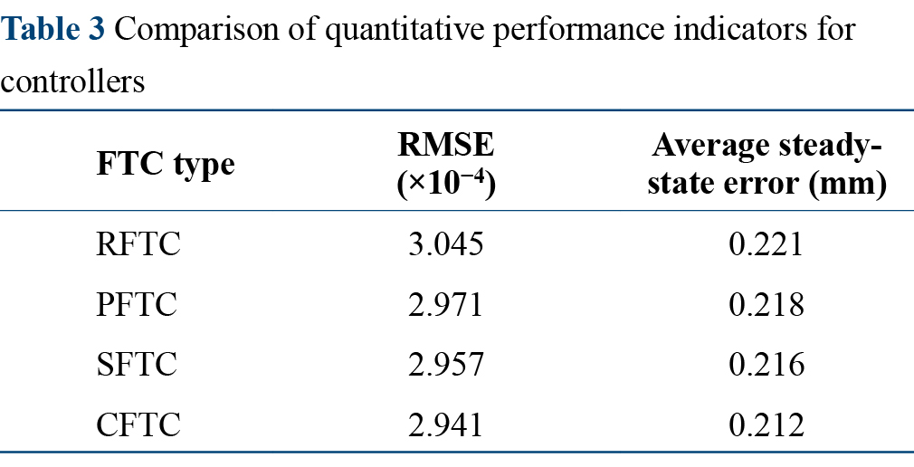
The proposed CFTC is compared with PFTC, SFTC, and a robust fault-tolerant controller (RFTC) using an SMO, as shown in Figure 8 and Table 3.
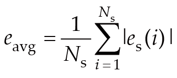
The average steady-state error is calculated as:(64)where es(i) denotes the tracking error at the i-th sampling instant within the selected steady-state interval, and Ns is the number of sampled data points in this interval.
After the occurrence of gain faults, the system controlled by the CFTC recovers to normal operation within 0.07 s, demonstrating fast recovery capability. The average steady-state error is 0.212 mm, with an RMSE of 2.941 × 10⁻⁴. Compared with PFTC, SFTC, and RFTC, the proposed CFTC achieves the lowest steady-state error and RMSE. This indicates that the CFTC effectively combines the advantages of different control strategies, achieving a better trade-off between performance and robustness. Therefore, the proposed CFTC improves the fault tolerance of the EMLA system and ensures reliable operation under fault conditions.
This paper proposes a fault diagnosis and CFTC scheme for the EMLA system based on an ISMLO. The main conclusions are summarized as follows:
(i) The proposed PD-type ISMLO achieves accurate fault detection and fault estimation, providing high-precision estimation with significantly reduced errors compared to conventional methods. The ISMLO enhances both robustness and estimation accuracy. Specifically, the sliding mode control law improves disturbance rejection capability, while the forgetting factor α enhances fault estimation by effectively utilizing historical information. As a result, the observer achieves fast convergence and high accuracy, which are essential for reliable fault estimation and fault-tolerant control.
(ii) The proposed CFTC strategy improves fault-tolerant performance by adaptively switching between PFTC and SFTC based on fault severity. This classification-based mechanism effectively combines their advantages, resulting in reduced steady-state error and improved robustness compared with individual controllers.
Overall, the proposed methods provide an effective solution for accurate fault diagnosis and reliable fault-tolerant control of EMLA systems under complex operating conditions.
Although the proposed ISMLO and CFTC strategies demonstrate strong performance in gain fault scenarios, the current study mainly focuses on actuator gain faults of the EMLA. More complex fault scenarios, such as bias faults, sensor faults, and compound faults, have not yet been fully considered. Therefore, further research is needed to extend the proposed framework to these fault types to enable more comprehensive fault diagnosis and fault-tolerant control in real-world systems. These extensions are expected to further enhance the robustness, adaptability, and control performance of the proposed framework in practical engineering applications.
Zhihao Hao: Conceptualization; methodology; software; validation; data curation; writing-original draft. Jiayu Lu: Conceptualization; supervision; project administration; funding acquisition; writing–review & editing. Bo Li: Methodology; formal analysis; writing–review & editing. Cao Tan: Software; validation; data curation; writing–review & editing. Huichao Zhang: Investigation; resources; validation; writing–review & editing. Ting Shu: Investigation; resources; data curation; writing–review & editing.
This work was supported by the National Natural Science Foundation of China (Grant Nos. 52305265, 52375105, and 52575298), and the National Key Research and Development Program of China (Grant No. 2024YFD2000101).
The data that support the findings of this study are available from the corresponding author upon reasonable request.
P. Song, M. Tomizuka, and C. F. Zong, "A Novel Integrated Chassis Controller for Full Drive-by-Wire Vehicles," Vehicle System Dynamics 53, no. 2 (2015): 215–236, https://doi.org/10.1080/00423114.2014.991331.
Z. X. Wang, C. N. Chen, Q. Jiang, H. Y. Zheng, and C. Kaku, "State Estimation of Drive-by-Wire Chassis Vehicle Based on Dual Unscented Particle Filter Algorithm," Chinese Journal of Mechanical Engineering 37, no. 1 (2024): 11, https://doi.org/10.1186/s10033-024-00993-y.
R. Azmi, M. Mirzaei, and A. Habibzadeh-Sharif, "A Novel Optimal Control Strategy for Regenerative Active Suspension System to Enhance Energy Harvesting," Energy Conversion and Management 291 (2023): 117277, https://doi.org/10.1016/j.enconman.2023.117277.
T. P. Yang, P. Q. Li, Q. P. Li, and Z. R. Li, "Active Suspension Control Strategy for Vehicles Based on Road Surface Recognition," Nonlinear Dynamics 112, no. 13 (2024): 11043–11065, https://doi.org/10.1007/s11071-024-09391-4.
X. T. Gao, Y. Du, S. Y. Han, et al., "Multi-Agent Reinforcement Learning for Vibration Control of Regenerative Active Suspension," Engineering Applications of Artificial Intelligence 153 (2025): 110809, https://doi.org/10.1016/j.engappai.2025.110809.
J. Y. Lu, B. Li, W. Q. Ge, C. Tan, and B. B. Sun, "Analysis and Experimental Study on Servo Dynamic Stiffness of Electromagnetic Linear Actuator," Mechanical Systems and Signal Processing 169 (2022): 108587, https://doi.org/10.1016/j.ymssp.2021.108587.
P. Yu, C. Tan, H. Yan, W. Q. Ge, Z. Y. Sun, and X. W. Chen, "Nonlinear Electromagnetic Force Analysis and Compensation Control of Electromagnetic Linear Actuator," Physica Scripta 98, no. 10 (2023): 105507, https://doi.org/10.1088/1402-4896/acf417.
H. Yan, Y. T. Lu, C. Tan, et al., "Multidisciplinary Optimization and Motion Control Method of Electromagnetic Linear Actuator for Electro-Hydrostatic System," Journal of the Brazilian Society of Mechanical Sciences and Engineering 46, no. 4 (2024): 200, https://doi.org/10.1007/s40430-024-04784-3.
C. Tan, H. X. Ren, B. Li, J. Y. Lu, D. X. Li, and W. M. Tao, "Design and Analysis of a Novel Cascade Control Algorithm for Braking-by-Wire System Based on Electromagnetic Direct-Drive Valves," Journal of the Franklin Institute 359, no. 16 (2022): 8497–8521, https://doi.org/10.1016/j.jfranklin.2022.09.006.
J. Y. Lu, C. F. Gu, Y. J. Zhao, C. Tan, Y. T. Lu, and C. Z. Fu, "Refined Modeling Method and Analysis of an Electromagnetic Direct-Drive Hydrostatic Actuation System," Actuators 11, no. 10 (2022): 281, https://doi.org/10.3390/act11100281.
Y. T. Lu, J. Y. Lu, C. Tan, M. W. Tian, and G. M. Dong, "Adaptive Non-Singular Terminal Sliding Mode Control Method for Electromagnetic Linear Actuator," Micromachines 13, no. 8 (2022): 1294, https://doi.org/10.3390/mi13081294.
T. J. Guo, S. Q. Chang, Z. Q. Chen, H. G. Huang, and J. T. Xu, "Fault Monitoring and Diagnosis of Actuators in Electromagnetic Valve-Train Based on Neural Networks Optimization Algorithm," IEEE Access 7 (2019): 110616–110627, https://doi.org/10.1109/ACCESS.2019.2933881.
M. Adamczyk and T. Orlowska-Kowalska, "Self-Correcting Virtual Current Sensor Based on the Modified Luenberger Observer for Fault-Tolerant Induction Motor Drive," Energies 14, no. 20 (2021): 6767, https://doi.org/10.3390/en14206767.
F. R. Kou, J. H. Wu, J. Gao, D. P. Wu, and R. C. Chen, "Active Fault-Tolerant Control Based on the Fault of Electromagnetic Hybrid Active Suspension," Shock and Vibration 2021, no. 1 (2021): 4273698, https://doi.org/10.1155/2021/4273698.
J. Li, X. X. Guo, C. Chen, and Q. Y. Su, "Robust Fault Diagnosis for Switched Systems Based on Sliding Mode Observer," Applied Mathematics and Computation 341 (2019): 193–203, https://doi.org/10.1016/j.amc.2018.08.036.
J. Xu, X. Wang, and Q. Y. Duan, "Active Fault Tolerant Control Based on Compound Iterative Learning Observer for Trajectory Tracking of Autonomous Underwater Vehicles," Ocean Engineering 286 (2023): 115540, https://doi.org/10.1016/j.oceaneng.2023.115540.
Q. L. Hu, B. Li, B. Xiao, and Y. M. Zhang, "Spacecraft Attitude Fault-Tolerant Control Based on Iterative Learning Observer and Control Allocation," in Control Allocation for Spacecraft under Actuator Faults (Singapore: Springer Singapore, 2021), 133–155, https://doi.org/10.1007/978-981-16-0439-3_7.
T. Kim, H. Jeong, and S. Kim, "Thrust-Fault Diagnosis of Hexacopter UAV Using Supervised Learning with Disturbance Observers," International Journal of Control, Automation and Systems 22, no. 12 (2024): 3570–3583, https://doi.org/10.1007/s12555-024-0532-x.
J. C. L. Chan, T. H. Lee, and C. P. Tan, "A Sliding Mode Observer for Robust Fault Reconstruction in a Class of Nonlinear Non-Infinitely Observable Descriptor Systems," Nonlinear Dynamics 101, no. 2 (2020): 1023–1036, https://doi.org/10.1007/s11071-020-05843-9.
R. C. Zhang, Z. W. Li, and W. Z. Liang, "Fault Detection and Identification for Rolling Mill Main Drive System Based on Integrated Observer under Iterative Learning Strategy," Proceedings of the Institution of Mechanical Engineers, Part I: Journal of Systems and Control Engineering 238, no. 4 (2024): 661–678, https://doi.org/10.1177/09596518231203110.
R. R. Wang and R. H. Chi, "Observer-Based Model-Free Iterative Learning for Fault-Tolerant Control of Nonlinear Systems," International Journal of Robust and Nonlinear Control 35, no. 13 (2025): 5506–5518, https://doi.org/10.1002/rnc.7995.
T. Yang, Y. T. Deng, H. W. Li, Z. Sun, H. Y. Cao, and Z. G. Wei, "Fast Integral Terminal Sliding Mode Control with a Novel Disturbance Observer Based on Iterative Learning for Speed Control of PMSM," ISA Transactions 134 (2023): 460–471, https://doi.org/10.1016/j.isatra.2022.07.029.
X. Wang, Y. Q. Zhou, and M. X. Liu, "Active Fault Tolerant Control Based on Adaptive Iterative Learning Observer against Time-Varying Faults in Thrusters of Autonomous Underwater Vehicle," Ocean Engineering 331 (2025): 121266, https://doi.org/10.1016/j.oceaneng.2025.121266.
F. L. Jia, F. F. Cao, G. R. Lyu, and X. He, "A Novel Framework of Cooperative Design: Bringing Active Fault Diagnosis into Fault-Tolerant Control," IEEE Transactions on Cybernetics 53, no. 5 (2023): 3301–3310, https://doi.org/10.1109/TCYB.2022.3176538.
Y. S. Hagh, R. M. Asl, A. Fekih, H. P. Wu, and H. Handroos, "Active Fault-Tolerant Control Design for Actuator Fault Mitigation in Robotic Manipulators," IEEE Access 9 (2021): 47912–47929, https://doi.org/10.1109/ACCESS.2021.3068448.
M. T. Gong, D. H. Zhou, L. Sheng, and X. He, "Multicontroller-Based Fault-Tolerant Control for Uncertain High-Order Sub-Fully Actuated Systems," IEEE Transactions on Cybernetics 55, no. 7 (2025): 3525–3536, https://doi.org/10.1109/TCYB.2025.3560406.
N. Xu, B. Niu, H. Y. Zhang, H. Q. Wang, G. D. Zong, and X. D. Zhao, "Hierarchical Sliding Mode Surface-Based Adaptive Neural Fault-Tolerant Control for Switched Nonlinear Systems with Average Dwell Time," Nonlinear Dynamics 111, no. 23 (2023): 21747–21763, https://doi.org/10.1007/s11071-023-08990-x.
M. L. Wang, J. Wang, and J. Huang, "Concomitant Observer-Based Multi-Level Fault-Tolerant Control for Near-Space Vehicles with New Type Dissimilar Redundant Actuation System," Symmetry 16, no. 9 (2024): 1221, https://doi.org/10.3390/sym16091221.
Y. T. Lu, C. Tan, W. Q. Ge, B. Li, and J. Y. Lu, "Improved Sliding Mode-Active Disturbance Rejection Control of Electromagnetic Linear Actuator for Direct-Drive System," Actuators 10, no. 7 (2021): 138, https://doi.org/10.3390/act10070138.
B. Jiang, M. Staroswiecki, and V. Cocquempot, "Fault Accommodation for Nonlinear Dynamic Systems," IEEE Transactions on Automatic Control 51, no. 9 (2006): 1578–1583, https://doi.org/10.1109/TAC.2006.878732.
L. P. Wang, D. H. Yuan, R. T. Cao, Q. Y. Zhang, and X. Yuan, "Automatic Landing of Carrier-Based Aircraft Based on a Collaboration of Fault Reconstruction and Fault-Tolerant Control," Aerospace Science and Technology 144 (2024): 108772, https://doi.org/10.1016/j.ast.2023.108772.
 Top
Top