2.1 Car-following model

During the development of traffic flow theory, numerous car-following models have been formed based on vehicle car-following theory [30]. Figure 1 shows the car-following scenario of vehicles on a single lane. Car-following theory is expressed through mathematical formulas or dynamic models, with the equation being:$\begin{array}{c}{\ddot{x}}_{n+1}(t+\text{Δ}t)=\lambda \left[{\dot{x}}_n(t)-{\dot{x}}_{n+1}(t)\right]\end{array}$(1)$\begin{array}{c}{v}_{n+1}(t+\text{Δ}t)={\dot{x}}_{n+1}(t)+{\ddot{x}}_{n+1}(t+\text{Δ}t)\text{Δ}t\end{array}$(2)$\begin{array}{c}{x}_{n+1}(t+\text{Δ}t)=x_{n+1}(t)+{\dot{x}}_{n+1}(t)\text{Δ}t+\frac{1}{2}{\ddot{x}}_{n+1}(t+\text{Δ}t){(\text{Δ}t)}^2\end{array}$(3)In the formulas, λ is response sensitivity coefficient (1 s⁻¹); x_n+1(t) is position of the (n + 1)-th vehicle at time t (m); x_n+1(t + Δt) is position of the (n + 1)-th vehicle at time t + Δt (m); ${\dot{x}}_n(t)$ is speed of the n-th vehicle at time t (m s⁻¹); ${\dot{x}}_{n\text{+1}}(t)$ is speed of the (n + 1)-th vehicle at time t (m s⁻¹); Δt is discrete time interval (s); ${\ddot{x}}_{n+1}$(t + Δt) is acceleration of the (n + 1) -th vehicle at time t + Δt (m s⁻²); v_n+1(t + Δt) is speed of the (n + 1) -th vehicle at time t + Δt (m s⁻¹).

Figure 1 Vehicle car-following schematic diagram

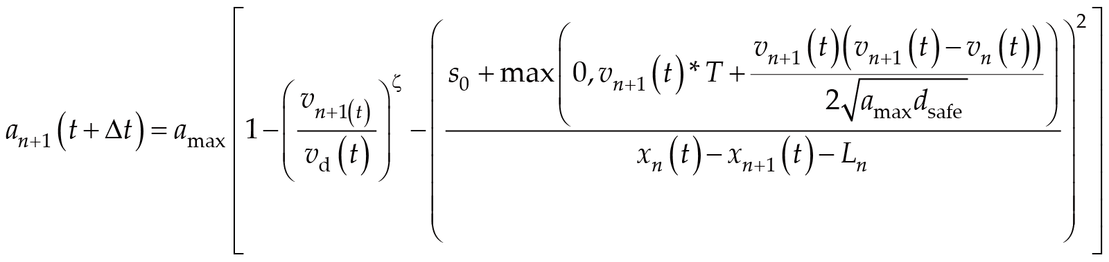
Based on this theory, intelligent driving car-following models consider the vehicle acceleration behavior of the subject vehicle under free-flow state and the safe car-following behavior when there is a leading vehicle. Treiber proposed the IDM model [31], which uses a unified model to describe vehicle car-following behavior under both free-flow and congested traffic flow states, with the output being vehicle acceleration. Its expression is:$\begin{array}{c}{a}_{n+1}\left(t+\text{Δ}t\right)=a_{\text{max}}\left[1-{\left(\frac{v_{n+1\left(t\right)}}{v_{\text{d}}\left(t\right)}\right)}^{\zeta }-{\left(\frac{s_0+max\left(0,v_{n+1}\left(t\right)*T+\frac{v_{n+1}\left(t\right)\left(v_{n+1}\left(t\right)-v_n\left(t\right)\right)}{2\sqrt{a_{\text{max}}{d}_{\text{safe}}}}\right)}{x_n\left(t\right)-x_{n+1}\left(t\right)-L_n}\right)}^2\right]\end{array}$(4)where: s₀ is minimum safe distance (m); T is safe time headway (s); v_d is desired velocity (m s⁻¹) ; ζ is acceleration exponent, generally taken as 4 (·); a_max is maximum acceleration (m s⁻²); d_safe is maximum comfortable deceleration (m s⁻²).

The IDM model, due to its clear parameter meanings, is widely used to simulate driving behavior on urban arterials [32], and is selected as the driving strategy for human-driven vehicles (HDV) [33]. Therefore, this paper adopts the IDM model to study vehicle car-following behavior on urban roads.

2.2 Lane-changing model

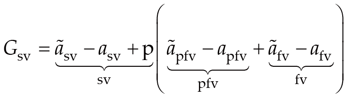
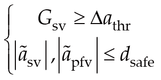
Compared to car-following behavior, vehicle lane-changing behavior is more complex and requires consideration of more factors [34]. Lane-changing behavior can be divided into three types: free lane-changing, cooperative lane-changing, and mandatory lane-changing. This paper focuses on analyzing whether drivers change lanes, so it concentrates on lane-changing decision models while ignoring the specific path of lane-changing. Rule-based models are one of the most fundamental lane-changing behavior frameworks, and the MOBIL lane-changing model is a rule-based lane-keeping judgment method [35]. This model considers factors such as the subject vehicle (SV), prospective following vehicle (PFV), following vehicle (FV), prospective leading vehicle (PLV), and leading vehicle (LV), as shown in Figure 2. It uses incentive criterion and safety criterion to judge whether to execute a lane-changing decision, takes comprehensive acceleration as the utility function, and aims at overall braking minimization. When the benefit of implementing lane-changing is greater than the expected benefit value and satisfies the safety criterion, it is considered that the driver executes the lane-changing action. The incentive criterion expression and safety criterion expression of the MOBIL model are, respectively:$\begin{array}{c}{G}_{\text{sv}}=\underset{\text{sv}}{\underbrace{{\tilde{a}}_{\text{sv}}-a_{\text{sv}}+\text{p}}}\left(\underset{\text{pfv}}{\underbrace{{\tilde{a}}_{\text{pfv}}-a_{\text{pfv}}}}+\underset{\text{fv}}{\underbrace{{\tilde{a}}_{\text{fv}}-a_{\text{fv}}}}\right)\end{array}$(5)$\begin{array}{c}\{\begin{array}{c}{G}_{\text{sv}}\ge \text{Δ}{a}_{\text{thr}}\\ \left|{\tilde{a}}_{\text{sv}}\right|,\left|{\tilde{a}}_{\text{pfv}}\right|\le d_{\text{safe}}\end{array}\end{array}$(6)In the formulas, ${\tilde{a}}_{\text{sv}}$ is acceleration of the subject vehicle after lateral lane-changing (m s⁻²); a_sv is acceleration of the subject vehicle before lateral lane-changing (m s⁻²); ${\tilde{a}}_{\text{sv}}$ is acceleration of the following vehicle in the target lane after the subject vehicle changes lane (m s⁻²); a_pfv is acceleration of the following vehicle in the target lane before the subject vehicle changes lane (m s⁻²); ${\tilde{a}}_{\text{sv}}$ is acceleration of the original following vehicle after the subject vehicle changes lane (m s⁻²); a_fv is acceleration of the original following vehicle before the subject vehicle changes lane (m s⁻²); p is yield coefficient (·); ∆a_thr is the minimum comprehensive acceleration benefit value that satisfies the subject vehicle's lateral lane-changing (m s⁻²); G_sv is the comprehensive acceleration benefit value of the subject vehicle after lateral lane-changing (m s⁻²).

Figure 2 Schematic diagram of subject vehicle lane-changing scenario in multi-lane traffic flow

The MOBIL model considers the adjacent relationships between vehicles when changing lanes and introduces a "politeness" coefficient to describe the cooperative behavior between vehicles during lane-changing. Since this model has clear logical relationships between variables and good parameter interpretability, this paper adopts the MOBIL model to study vehicle lane-changing behavior on urban roads.

2.3 Driver behavior prediction model

In microscopic traffic, vehicles on the road are typically self-driven individuals with interconnected effects [36]. Driver driving behavior and vehicle motion characteristics converge into orderly moving traffic flow. Building upon the vehicle's current motion state, the driver behavior prediction model intelligently simulates future driving behavior and decision-making processes of human drivers. The simulation process considers the interaction between surrounding vehicles and the subject vehicle as well as the influence of traffic signal status on driver behavior, predicting vehicle state changes over a future period of time. Based on the simulated traffic conditions, vehicle queue prediction ahead of intersections is realized, and calculations of indicators such as the maximum number of queued vehicles and queue dissipation time are performed.

Vehicles have randomness in spatiotemporal distribution. To facilitate problem research, certain assumptions are made about actual traffic. The assumptions include:

(1) Road vehicles are homogeneous with a consistent vehicle body length;

(2) Drivers are assumed to be homogeneous and follow a unified driving behavior model;

(3) Only free lane-changing behavior is considered, assuming vehicles on through arterials do not perform turning, U-turn, or other behaviors;

(4) Front and rear vehicles in the same lane have car-following relationships.

The IDM mentioned in section 2.1 is a calculation function for vehicle acceleration that does not consider the influence of traffic signals on vehicle driving behavior in urban traffic. To make IDM more applicable to urban road networks, green light countdown and red light remaining time information at intersections are introduced into the model. The mathematical expression of the improved IDM model is:$\begin{array}{c}{\ddot{x}}_{n+1}(t)=f\left(x_{n+1}(t),x_n(t),t_{\text{gl}},t_{\text{rl}}\right)\end{array}$(7)where t_gl is the remaining green light duration, t_rl is the remaining red light duration. The IDM model, improved in this way, considers the influence of traffic signals on the driving state of vehicles closest to the intersection, making it more applicable to actual urban road network conditions.

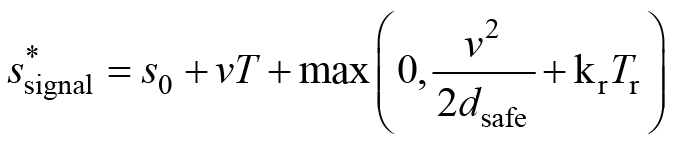
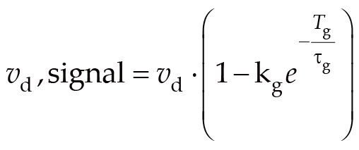
In the improved IDM formulation, the remaining green time T_g and remaining red time T_r directly influence the driver's longitudinal decision process when approaching an intersection. Specifically, the signal information is incorporated into the IDM through the desired gap term, which governs the deceleration behaviour when a red phase is imminent. The desired dynamic gap is modified as follows:$\begin{array}{c}{s}_{\text{signal}}^{*}=s_0+vT+\max \left(0,\frac{v^2}{2d_{\text{safe}}}+{\text{k}}_{\text{r}}{T}_{\text{r}}\right)\end{array}$(8)where k_r (set to 2.0 in this study based on empirical trials) is a sensitivity coefficient representing the driver's tendency to begin braking earlier when the remaining red time is long. The additional term increases the effective desired gap and therefore reduces the acceleration output of the IDM, resulting in anticipatory braking. Conversely, when the remaining green time T_g is short, the desired speed v_d of the IDM is adjusted downward smoothly according to:$\begin{array}{c}{v}_{\text{d}},signal=v_{\text{d}}\cdot \left(1-{\text{k}}_{\text{g}}{e}^{-\frac{T_{\text{g}}}{{\text{τ}}_{\text{g}}}}\right)\end{array}$(9)where k_g (taken as 0.5) and τ_g (taken as 3.0 s) regulate the strength and time scale of the adjustment, representing the intensity of acceleration reduction and the anticipation horizon for the yellow phase, respectively. This mechanism reflects the common driving behaviour whereby drivers avoid unnecessary acceleration when a green light is about to end. These additions explicitly embed the influence of upcoming signal changes into the IDM, enabling the model to better reproduce the characteristic start-stop process at signalized intersections.

Each driver is treated as an independent decision-making entity. Any single vehicle serves as the SV in sequence. Based on the improved IDM car-following model combined with the MOBIL lane-changing model, the possibility of the subject vehicle changing to adjacent lateral lanes is considered, with the allowable offset amount per lateral lane-changing specified as one lane. The two possible situations of SV lane-changing and not lane-changing are represented using a lane-changing index, where L_C = 0 represents not changing lanes, and L_C = 1 represents changing lanes. The lane where SV is currently located is called the ego lane, and the adjacent lateral lane with lane-changing probability is called the target lane. In the ego lane, the vehicle closest to SV ahead of SV in longitudinal displacement is called the ego lane leading vehicle, and the vehicle closest to SV behind SV is called the ego lane following vehicle; in the target lane, the vehicle closest to SV ahead of SV in longitudinal displacement is called the target lane leading vehicle, and the vehicle closest to SV behind SV is called the target lane following vehicle.

Considering a two-lane scenario, the surrounding traffic environment of SV can be divided into four situations in both longitudinal and lateral displacement. Ego lane: having both leading and following vehicles, having a leading vehicle but no following vehicle, having a following vehicle but no leading vehicle, having neither leading nor following vehicle. Target lane: having both leading and following vehicles, having a leading vehicle but no following vehicle, having a following vehicle but no leading vehicle, having neither leading nor following vehicle. When SV changes lanes, it affects surrounding vehicles. Whether the target lane leading vehicle exists and the longitudinal spacing between SV and the target lane leading vehicle affect lane-changing benefits; whether the target lane following vehicle exists and the longitudinal spacing between SV and the target lane following vehicle affect lane-changing safety; whether the original lane leading vehicle exists affects lane-changing motivation; whether the original lane following vehicle exists affects lane-changing cooperative benefits. As shown in Figure 3, in a two-lane scenario, there are sixteen types of surrounding vehicle traffic environment situations that affect whether the SV executes lane-changing behavior.

Figure 3 Classification of the surrounding traffic environment for the lane-changing subject vehicle in a two-lane scenario

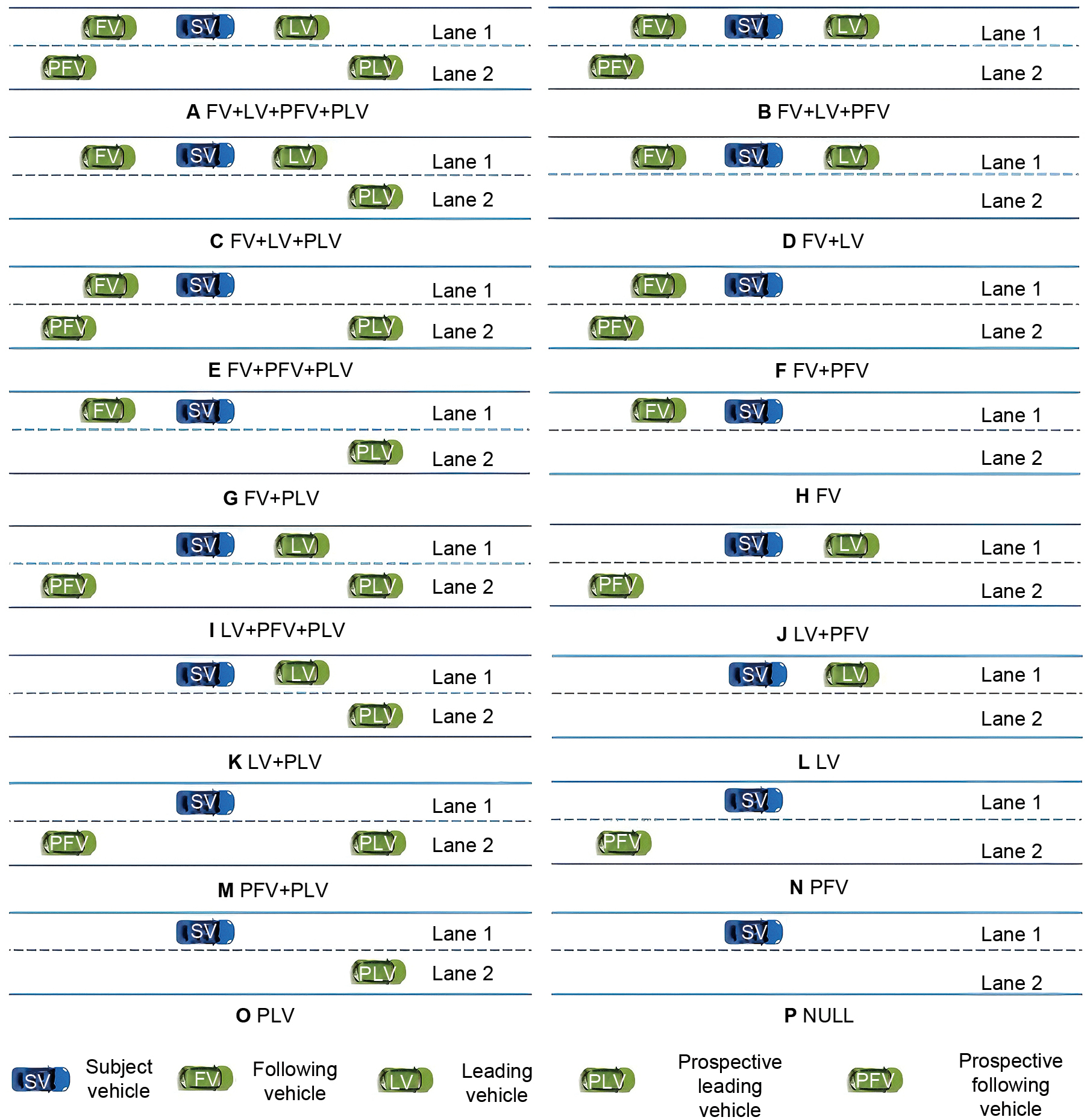
Although Figures 2 and 3 illustrate the interaction structure in a two-lane scenario for clarity, the proposed driver-behavior prediction framework is not restricted to two lanes. For an approach with N lanes, the same procedure is applied by evaluating the IDM–MOBIL rules with respect to all adjacent candidate lanes. The identification of leading and following vehicles, the lane-changing incentive calculation, and the safety criterion naturally extend to a multi-lane structure without altering the core formulation. The two-lane diagrams are used solely for illustrative purposes.

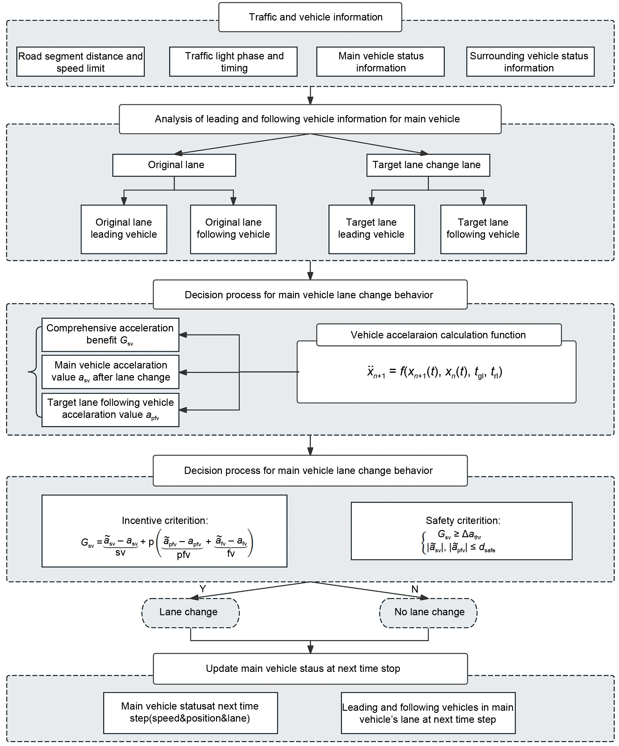
The driver behavior prediction model consists of five parts: traffic flow state initialization, traffic signal phase update, judgment of whether vehicles maintain car-following or change lanes in the next time unit, vehicle acceleration calculation, and vehicle speed and position update for the next time unit. The prediction of SV's motion state over a future period uses Δt as the basic time unit. Within a single time unit, SV makes decisions by judging the status of surrounding traffic vehicles and traffic signals, predicting SV's lane-changing or car-following behavior at the next moment. First, based on vehicle information in matching lanes, the front and rear vehicle information in SV's original lane and target lane are identified. According to the search results and the front-rear relationship between vehicle positions and SV position, the current existence of leading and following vehicles in SV's ego lane and target lane is analyzed, determining which situation in Figure 3 the current SV's surrounding traffic conditions belong to. Then, the improved IDM model is used to calculate the acceleration values of the subject vehicle, original lane following vehicle, and target lane following vehicle after the SV driver intends to change lanes. The comprehensive acceleration benefit assuming SV lane-changing is calculated according to Equation (5), and based on this value, judgment is made according to the criterion in Equation (6), whether the subject vehicle will change lanes at the next moment. When G_sv is exceeded, and lane-changing satisfies safety conditions, it is considered that SV will choose to change lanes. If either condition is not satisfied, it is considered that SV maintains car-following driving. Car-following driving calculation includes a free road acceleration term, a deceleration term for maintaining a safe distance from the front vehicle, and a speed adjustment term for smoothly approaching the intersection stop line during red signal phases.

All acceleration term calculations in the prediction are based on the improved IDM model, updating the subject vehicle's speed, position, and lane information for the next time unit according to the composition structure in Figure 4. Based on sensing facilities deployed roadside, real-time vehicle state information is periodically obtained, acquiring acceleration, speed, longitudinal position, and lane position information for each sensed vehicle. Then, a discrete prediction mechanism with time stepping is adopted, inheriting the calculated SV vehicle motion state attributes for the next moment, continuously updating SV speed and position, and storing corresponding state attributes in each time unit, thereby deducing the change process of SV's motion state (such as acceleration, speed, lane location, etc.) over a future period of time.

Figure 4 Schematic diagram of the driver-behavior prediction model

3.1 Vehicle traffic scenarios at signalized intersections

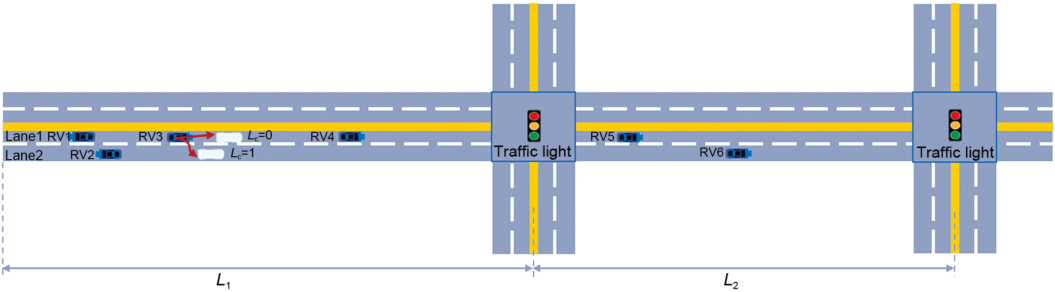
This section studies the problem of predicting vehicle queue accumulation and queue dissipation time ahead of signalized intersections in urban road segment scenarios. Figure 5 shows an urban road scenario with two lanes at consecutive signalized intersections.

Figure 5 Two-lane urban road scenario with consecutive signalized intersections

The road segment in Figure 5 is presented as a two-lane configuration, but the queue-prediction mechanism is applicable to any number of lanes because queue accumulation and dissipation are evaluated on each lane independently.

This route contains two consecutive signalized intersections with information attributes including L_i, N_lane, v_limit. L_i is the geometric length of the i-th road segment, N_lane is the number of lanes, and v_limit is the maximum speed limit for road driving.

Traffic signal phase and timing information attributes include $t_{\text{r}}^i,t_{\text{g}}^i,t_{\text{y}}^i,p_{\text{ini}}^i$ and $t_{\text{offset}}^i$. $t_{\text{r}}^i,t_{\text{g}}^i,t_{\text{y}}^i$ are the durations of red light, green light, and yellow light respectively within one signal cycle of the i -th road segment. $p_{\text{ini}}^i$ is the initial phase of the i-th road segment, and $t_{\text{offset}}^i$ is the offset time of the i-th road segment relative to the initial phase. Road vehicles (RV) information attributes include $N_{\text{rv}},A_{\text{rv}}^j,V_{\text{rv}}^j,X_{\text{rv}}^j,T_{\text{rv}}^j$ and $L_{\text{rv}}^j$. N_rv is the number of road vehicles within the sensing range of roadside equipment at the current moment, where vehicles are assigned a sequence number j=1,2,…,N_rv in the west-to-east direction. $A_{\text{rv}}^j,V_{\text{rv}}^j,X_{\text{rv}}^j,T_{\text{rv}}^j$ and $L_{\text{rv}}^j$ are respectively the acceleration, speed, position, time of entering the current road segment, and lane position of the j-th vehicle among road vehicles.

3.2 Queue process analysis

Without considering vehicle queuing problems caused by non-signal phase alternation, when the traffic signal at the intersection ahead in the vehicle's driving direction is in red phase, drivers have the obligation to comply with traffic rules and often gradually reduce their driving speed, eventually stopping at the intersection stop line and waiting for the next green light to turn on. Before this, vehicles from upstream road segments will successively arrive at this road segment and gradually stop and wait, forming a queue.

The key to identifying different traffic flow state transition points lies in vehicle driving speed. Traffic queuing can be divided into three states:

(1) Queue formation: during red signal periods, the number of queued vehicles increases with the increase in vehicle arrival flow;

(2) Queue stagnation: due to red signals on upstream road segments preventing traffic flow from continuing to arrive, the queued vehicle queue remains stable;

(3) Queue dissipation: when green signals turn on, the number of queued vehicles gradually decreases with the increase in vehicle arrival flow.

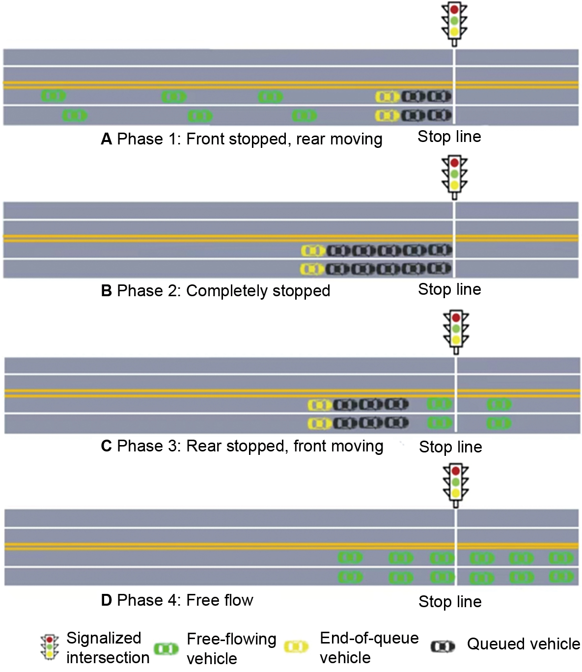
The above three states can be summarized into four phases, as shown in Figure 6: (i) front vehicles stop, rear vehicles move; (ii) complete stop; (iii) rear vehicles stop, front vehicles move; (iv) all vehicles are moving freely. Green vehicles represent normally flowing vehicles, black vehicles represent vehicles already in a queuing state, and yellow vehicles represent the tail vehicle in the queued vehicle group.

Figure 6 Complete process of traffic queue formation and dissipation

Analyzing Figure 6, during the process of upstream vehicles gradually approaching the intersection, since the intersection ahead is still in a red light window and the earliest stopped and waiting vehicles have not yet been released, hindered by front vehicles, rear vehicles also need to gradually reduce their driving speed. Finally, under the condition of maintaining a certain safe distance from front vehicles, they join the queued stopped vehicle group, thus forming the queuing phenomenon in road traffic. Before the traffic signal at the intersection ahead turns green, if the upstream intersection remains in a passable state, queued vehicles will continue to accumulate. When the traffic signal on the upstream road segment turns to the red phase, it will block the arrival of the current road segment traffic flow, at which time the vehicle queue neither increases nor decreases. As time progresses, the traffic signal at the intersection ahead becomes green, and the front-most vehicles in the queue start first, with rear vehicles starting successively after the leading vehicle with a delay. The starting phase has lag characteristics. Since tail vehicles need to wait for their front vehicles to start before they can start, the rear of the queue is still in a queuing state at this time. The vehicle queuing process approximates stopping waves arriving at tail vehicles sequentially from front to back, and the vehicle starting process approximates starting waves arriving at tail vehicles from front to back. Usually, the transmission speed of starting waves is higher than that of stopping waves. When the two waves meet, the entire traffic flow will change from a queued stagnation state to a normal traffic state.

3.3 Vehicle queue and dissipation time prediction algorithm

Different from occasional deceleration behavior during vehicle driving, typically during the process of vehicles transitioning from a normal driving state to a stopped queuing state, the driving speed will remain at low values within a certain time range. The highway capacity manual (HCM) stipulates that any single vehicle with a speed below 3 m s⁻¹ or stopped or following behind already queued vehicles is considered a queued vehicle. In this study, a vehicle is regarded as being in a queued state when its instantaneous speed falls below 5 km h⁻¹. A threshold of 5 km h⁻¹ is adopted to identify queued vehicles, consistent with default settings in SUMO and ensuring uniformity across both simulation and field data analysis.

All vehicles entering this intersection need to stop and wait in order of arrival before the intersection stop line, before the traffic signal turns green. Based on the driver behavior prediction model established in section 2.3, motion state changes of each microscopic vehicle at the next moment are predicted within the same time step, and based on the predicted next-moment vehicle state from the previous moment as the initial state of vehicles at the next moment, step-by-step iterative prediction is performed for each of the above microscopic vehicles, thereby realizing deduction of future traffic situations. When deducing the time-space curves during the process of road vehicles passing through intersections, the predicted acceleration value, speed value, displacement value, and vehicle lane position of each road sensing vehicle at each prediction time step are stored. Meanwhile, within continuous multiple time steps, it is judged whether the predicted driving speed of vehicles is less than the set stopping speed. If satisfied, the vehicle IDs are stored in the queued vehicle ${\text{RV}}_{\text{queue}}^{i,l,r}\left\{r=1,2,\mathrm{...},m\right\}$ containing at least one element. This queued vehicle distinguishes different intersections and different lanes of the same intersection, where the contained elements are vehicle IDs that will exhibit stopping behavior ahead of intersections during future red lights.

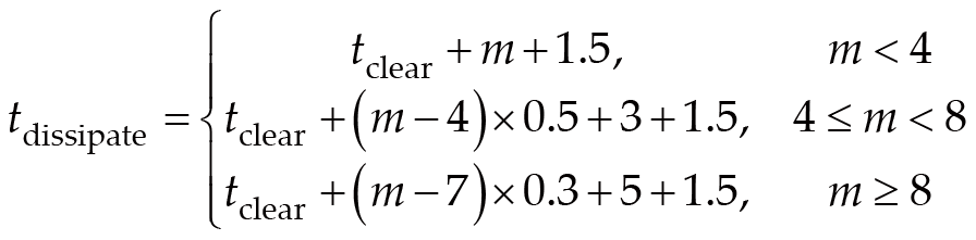
Queued vehicles ahead of intersections follow the "first-in-first-out" principle. According to the queued vehicle ${\text{RV}}_{\text{queue}}^{i,l,r}$, when determining vehicles in stagnation state during the vehicle queuing process forming a stable queue, the vehicle positioned furthest back and farthest from the intersection stop line among stopped vehicles is identified. This vehicle is the queue tail vehicle ${\text{RV}}_{\text{queue}}^{i,l,m}$ ahead of the stop line in the current lane of this intersection. The number of vehicles included from the queue tail vehicle to the queue head vehicle is the maximum number of queued vehicles m in the current lane of the current intersection during the next red light. After determining the queue tail vehicle, the predicted speed sequence and predicted displacement sequence of the predicted queue tail vehicle are analyzed intersection by intersection and lane by lane. According to the predicted speed sequence of the queue tail vehicle, the moment $t_{\text{pass}}^{i,l,o}$ when the tail vehicle enters the intersection, and the distance from the intersection stop line when in queuing waiting state are determined. This distance is the predicted maximum queue length value for the current lane of the current intersection during the next red light period. When queued vehicles transition from the stopped state to the starting state, different vehicles have varying starting performance, initial vehicle positions, and driver reaction times, which will form different degrees of stopping delay and acceleration delay. Some related domestic studies indicate that vehicles in the first position have the greatest impact on starting loss, followed by the next few vehicles, with decreasing influence. To ensure vehicle driving safety, a certain headway should be maintained between front and rear vehicles, typically 1.5 s. To incorporate a safety time margin, a segmented calculation is performed according to the maximum number of queued vehicles. The formula for calculating queue dissipation time is given as follows.$\begin{array}{c}{t}_{\text{dissipate}}=\{\begin{array}{cc}{t}_{\text{clear}}+m+1.5,& m<4\\ t_{\text{clear}}+\left(m-4\right)\times 0.5+3+1.5,& 4\le m<8\\ t_{\text{clear}}+\left(m-7\right)\times 0.3+5+1.5,& m\ge 8\end{array}\end{array}$(10)

In Equation (10), t_clear represents the time interval between the moment when the tail vehicle of the queue passes the stop line and the onset of the next green phase. This interval forms the base clearing time before the start-up wave propagates through the queued vehicles. The piecewise coefficients in the equation reflect empirically observed differences in start-up wave propagation speeds for short, medium, and long queues in typical urban traffic, where short queues dissipate faster while longer queues accumulate additional acceleration and reaction delays.

To improve readability and interpretability, the meaning of Equation (10) is further clarified as follows. The total dissipation time consists of two components: (i) the clearing time, and (ii) the start-up wave propagation time. The latter is approximated by three piecewise linear segments based on observed driver behaviour: rapid propagation for small queues (m < 4), moderate delay for medium queues (4 ≤ m < 8), and slower propagation for long queues (m ≥ 8). For example, when the queue length is m = 6, the model selects the middle segment (4 ≤ m < 8), yielding: t_dissipate = t_clear + (m – 4) × 0.5 + 3 + 1.5.

Here, (m – 4) × 0.5 corresponds to the additional interaction delay of the extra vehicles, while the base start-up time (3 s) and safety headway (1.5 s) represent typical acceleration and spacing patterns at intersections. This example illustrates the physical meaning of each term and the rationale behind the piecewise formulation.

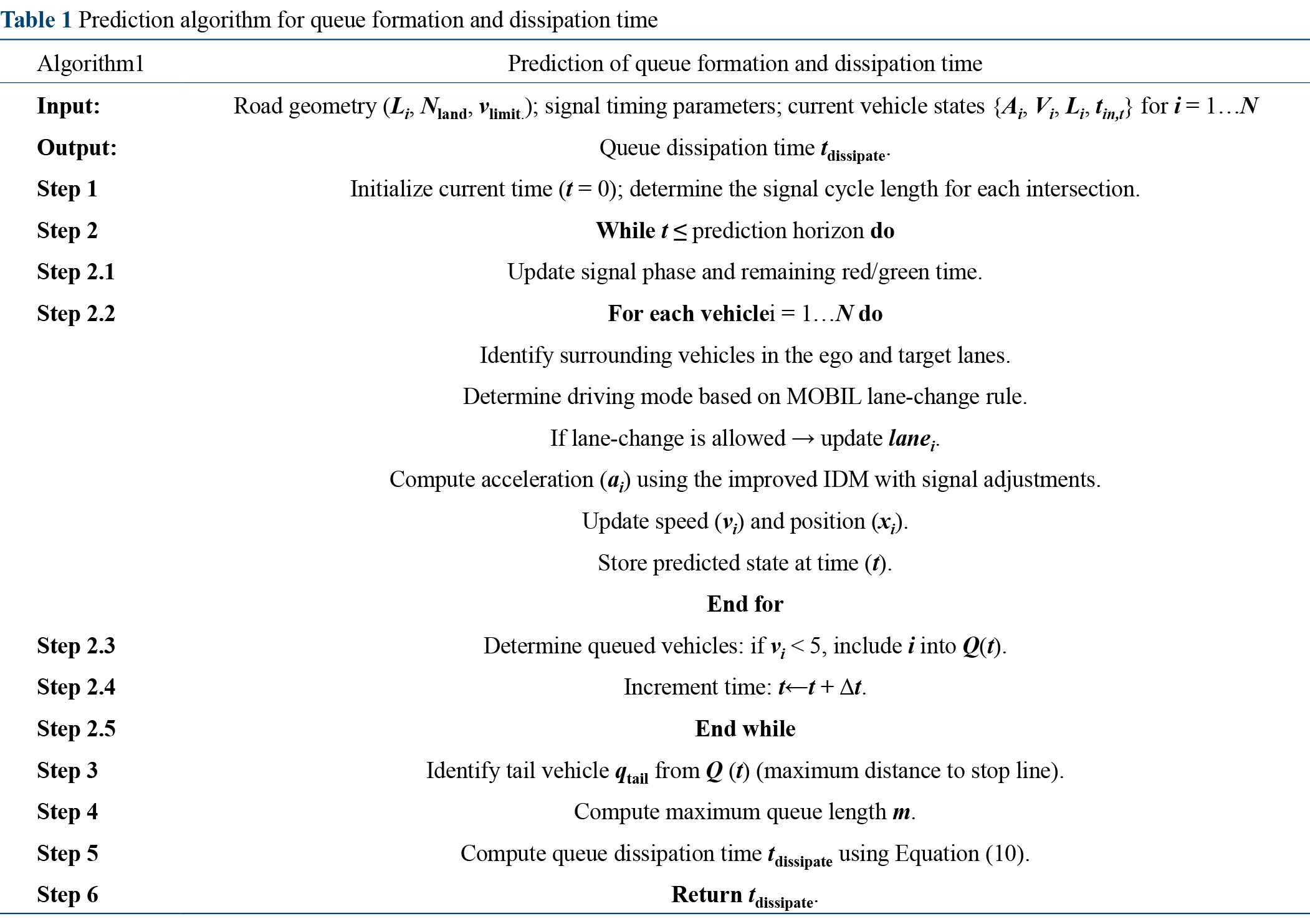
After computing the dissipation time, the full prediction procedure for queue formation and dissipation can be summarized in the algorithm presented below (Table 1).

The algorithm operates in discrete time steps and predicts the future motion of each detected vehicle until the moment when the next red phase ends. At each time step, the algorithm (i) updates signal timing information; (ii) determines whether each vehicle is in free-driving, car-following, or lane-changing mode based on the IDM-MOBIL rules; (iii) computes acceleration and updates speed and position; and (iv) checks whether the vehicle's speed falls below the queue threshold, thereby marking its participation in the future queue. After iterating through all vehicles and time steps, the algorithm identifies the tail vehicle, computes the maximum queue length, and finally derives the queue dissipation time using Equation (10).

Due to the extremely strong time-varying characteristics of real traffic, errors in long-term traffic prediction processes will gradually accumulate. Therefore, this prediction process adopts an iterative update mechanism that receives real-time position and state information of road vehicles from roadside sensing according to a certain update frequency. All prediction processes are completed in one algorithm calculation until triggering the next update of real road vehicle position and state information, and executing the second prediction, cyclically and repeatedly updating the prediction process of road vehicles passing through intersections in the future.

4.1 Simulation setup

A unidirectional urban arterial two-lane route with two consecutive intersections is set up, with road segment start/end points divided by intersection center points, as shown in Figure 7. The displacement values of stopping points use the starting point of road segment one as reference, and vehicles stop for 25 s at both the starting and ending stopping points, respectively. Both intersections start with red signal phases, with red light timing of [54, 56] seconds from front to back sequentially, green light timing of [56, 54] seconds, and a simulation time of 360 seconds.

Figure 7 Simulation road segment design

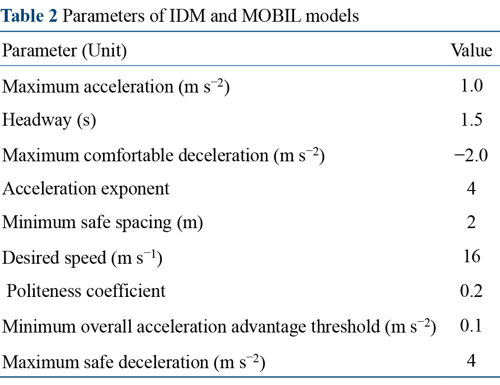
By modeling the above road traffic scenario in SUMO and simultaneously establishing a traffic signal control system, random traffic flow is generated by assigning different traffic flow volumes. Electric buses within the traffic flow are designated as subject vehicles, while other traffic environment vehicles are surrounding vehicles, assuming all surrounding vehicles have a body length of 5 m. The car-following behavior of surrounding vehicles follows IDM, and the lane-changing model follows LC2013. Key parameters for IDM and MOBIL are listed in Table 2, where IDM settings follow [36], MOBIL settings follow [37].

4.2 Queue prediction model verification

When inputting each group of traffic flow volume simulation runs, by scrambling random factors, the driving behavior of each vehicle in the input road segment traffic flow also changes randomly, satisfying the randomness of real traffic as much as possible. The maximum number of queued vehicles observed at intersections in nine simulation experiments is selected for comparison with model-predicted values. Observed values are obtained based on traffic vehicle states captured by lane area detectors in different lanes of each road segment in SUMO, similar to real-time roadside equipment in the real world. Current road vehicle state data is obtained through roadside equipment, and a certain moment is randomly selected. Based on road vehicle state information received at that moment, future driving trajectories of sensed vehicles are predicted, and the queue estimation method is verified using the maximum number of queued vehicles ahead of intersection stop lines as an indicator. The maximum number of queued vehicles in different lanes at each intersection within the most recent signal cycle is predicted, respectively, with the current moment as the time starting point.

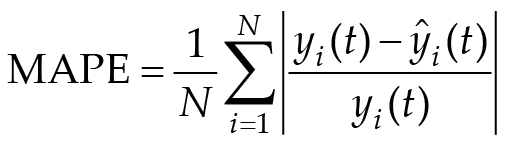
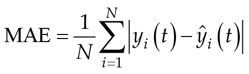
Since traffic flow lacks stability when first entering road segments, traffic flow in downstream road segments requires upstream vehicles to arrive successively after a period of time. Therefore, the cycle after traffic flow stabilization in the second road segment is selected as the observed value. Here, results at the end of the second red light cycle after simulation start (236 s) are selected for statistical comparison. Model evaluation indicators use mean absolute error (MAE) and mean absolute percentage error (MAPE). The calculation formulas for MAE and MAPE are, respectively:$\begin{array}{c}\text{MAPE}=\frac{1}{N}\end{array}{\displaystyle \sum _{i=1}^N\left|\frac{y_i(t)-{\widehat{y}}_i(t)}{y_i(t)}\right|}$(11)$\begin{array}{c}\text{MAE}=\frac{1}{N}\end{array}{\displaystyle \sum _{i=1}^N\left|y_i\left(t\right)-{\widehat{y}}_i\left(t\right)\right|}$(12)where, N is the number of observed values, y_i(t) is the true value of the maximum number of queued vehicles at time t, and y_i(t) is the estimated value of the maximum number of queued vehicles at time t.

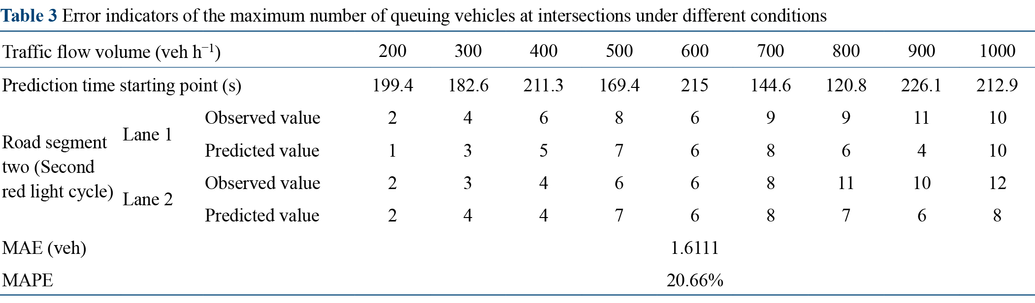
The length of the prediction horizon and the traffic demand level have significant impacts on the estimation results. Using the simulation start time as the origin, subsequent prediction instants are defined relative to this origin. Table 3 reports the MAE and MAPE of maximum queue length prediction for the proposed method under nine demand levels. Under light-to-medium demand (200–700 veh h⁻¹), the predicted values remain close to the simulated ground truth, with relatively small errors.

Under light-to-medium demand levels, most vehicles that eventually participate in queuing have already entered the approach at the beginning of the prediction horizon. In these cases, the queue evolution is dominated by signal-induced stopping behaviour, which is well represented by the signal-aware IDM. In contrast, under high-demand conditions (800–1,000 veh h⁻¹), two factors contribute to increased prediction errors. First, in near-saturated traffic, drivers exhibit larger fluctuations in acceleration and speed adaptation, making their behaviour more difficult to characterise using a deterministic car-following model. Second, in scenarios where the prediction horizon begins earlier (e.g., the 800 veh h⁻¹ case), additional upstream vehicles that arrive later in the cycle are not observed at the prediction start time, leading to systematic underestimation of the maximum queue length. These factors jointly explain the larger errors observed in Table 2 for high-demand scenarios.

These observations also suggest several directions for improvement. For congested conditions, the car-following component may be extended with state-dependent parameters or mild stochastic perturbations so that driver behaviour under near-saturated flow is represented more accurately. To reduce the underestimation caused by vehicles entering the approach after the prediction start time, a rolling or updated prediction horizon based on upstream detector information could be adopted. In addition, incorporating upstream inflow information or corridor-level coordination into the framework would help capture multi-intersection interactions in future studies.

The nine simulation scenarios in Table 2 cover off-peak, medium, and near-saturated traffic conditions with arrival flows ranging from 200 to 1,000 veh h⁻¹ per direction. For each demand level, different signal timing settings are tested to represent typical off-peak and peak-period operation at urban intersections. The simulated road geometry adopts the same two-lane approach configuration as the Yizhuang field site, allowing the microscopic behaviour model to be validated under comparable lane structures. The results indicate that the proposed method maintains good prediction performance across different demand levels and signal cycles, particularly in medium and high demand scenarios that are critical for green-wave coordination.

4.3 Baseline comparison

To further clarify the performance of the proposed method, two representative baseline models were implemented for comparison. The first is a shockwave-based model ("Shockwave"), in which a macroscopic queue-estimation formulation is constructed using the backward shockwave speed derived from the Greenshields model, following Gao et al. [10]. This model represents pure signal–arrival-flow logic without any microscopic driving behaviour and is widely used as a conventional benchmark for queue estimation.

The second baseline is a data-driven predictor based on SVR. For this model, a total of 114 labelled samples were extracted from the simulation dataset, with each sample corresponding to one signal cycle and its associated maximum queue length. Aggregated traffic-flow and signal-timing features were used as input variables, and the maximum queue length of each cycle served as the prediction target. The samples were randomly divided into 80% for training and 20% for testing, and the training was repeated for 50 shuffled partitions to reduce variance arising from the limited dataset. A radial basis function kernel was adopted, and the hyperparameters (C, γ) were tuned via grid search. This baseline characterises short-term queue formation purely from historical cycle-level patterns, without explicitly modelling driver behaviour or signal–behaviour interactions.

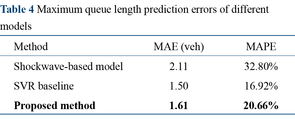
Table 4 summarises the MAE and MAPE of maximum queue length prediction for the Shockwave model, the SVR baseline, and the proposed method across all simulated scenarios. The Shockwave-based estimator yields the largest errors, reflecting the limitations of using a constant backward wave speed and neglecting microscopic driver responses to signal countdowns. The SVR baseline achieves the lowest MAPE by directly learning from labelled samples in the simulation dataset. However, its applicability is constrained by the need for sufficient training data and retraining whenever traffic demand patterns or signal settings change. The proposed behaviour-based method attains an intermediate error level, while remaining fully interpretable and not requiring historical data or model retraining for new scenarios. From an engineering perspective, this offers a practical trade-off between accuracy, data dependency, and deployment effort.

5.1 Verification road

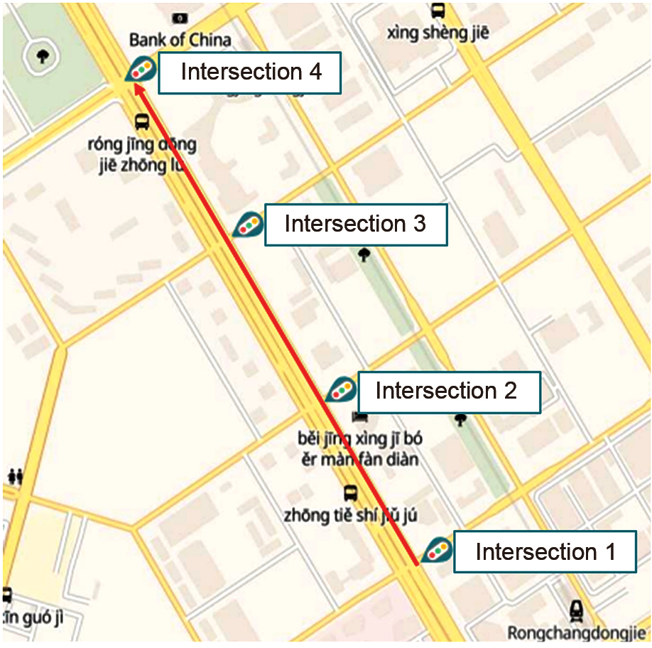
Different from the simulation-based verification in section 4.2, this section evaluates the proposed method using roadside sensing data collected along the operating route of Bus Line 846 in Yizhuang District, Beijing. The verification road segment lies between the Ronghua Road South Ring Island North Station and the Rongjing East Street West Entrance Station, with a posted speed limit of 60 km h⁻¹. The spatial layout of the study corridor is illustrated in Figure 8, where red arrows indicate the forward traffic direction. The route contains four signalised intersections—Ronghua Road–Jinxiu Street, Ronghua Road–Yuncheng Street, Ronghua Road–Xingsheng Street, and Ronghua Road–Rongjing East Street—forming three consecutive arterial segments.

Figure 8 Verification road segment

Field observations were conducted from 16:00 to 17:00 on a weekday afternoon peak period. During this one-hour interval, the roadside sensing system continuously recorded vehicle trajectories and signal-state information, covering 36 complete signal cycles. For each cycle, the lane-based maximum queue length at the end of the red phase was extracted. After removing incomplete cycles and abnormal detections, a total of 512 valid queue samples were obtained and used for model evaluation.

Unlike the simulation experiments that assume a unified signal plan, the three downstream intersections along the verification corridor operate under different signal-timing settings and different initial signal states. Table 5 summarises the signal timing parameters for the three consecutive approaches in the direction of vehicle travel. The table provides (i) the initial signal phase at the moment of observation, (ii) the initial phase offset (remaining time of the current phase), and (iii) the durations of the red, green, and yellow phases for each intersection. The approach at the studied downstream segment contains two through lanes, which matches the lane configuration adopted in the simulation experiments and enables direct comparison between simulated and real-world queue evolution.

g denotes a green initial signal phase; r denotes a red initial signal phase. The initial phase offset represents the remaining duration of the current phase at the observation start time. The three intersections operate independently, and their heterogeneous timings are fully considered in field verification.

5.2 Model verification

The accuracy of vehicle queue prediction plays a key role in the execution effectiveness of green-wave speed planning. Therefore, this study verifies the effectiveness of the behaviour-based prediction model by comparing roadside-sensed queuing conditions with the predicted queue states. To calibrate the car-following parameters of the IDM, 40 pairs of front–rear vehicles with stable car-following behaviour were selected from the preprocessed roadside-sensing dataset. The trajectories were divided into 80% for calibration and 20% for validation.

For each selected vehicle pair, the trajectory of the leading vehicle served as the input, and the five IDM parameters (maximum acceleration, comfortable deceleration, desired headway, minimum safe spacing, and desired speed) of the following vehicle were calibrated by minimizing the discrepancy between the simulated and observed trajectories. The objective function was defined as a weighted mean absolute error combining speed and spacing:$\begin{array}{c}ℒ=\text{α}\cdot \text{MAE}\left(v_{\text{sim}},v_{\text{obs}}\right)+\left(1-\text{α}\right)\cdot \text{MAE}\left(s_{\text{sim}},s_{\text{obs}}\right)\end{array}$(13)where α = 0.6 was chosen to place slightly greater emphasis on reproducing speed profiles. The genetic algorithm (GA) was configured with a population size of 120, 200 generations, tournament selection, and Gaussian mutation. Bounds for the IDM parameters followed typical values reported in previous studies. Because the GA is stochastic, the procedure was repeated 20 times, and the mean of the resulting parameter sets was taken as the calibrated value. The calibrated parameters are listed in Table 6.

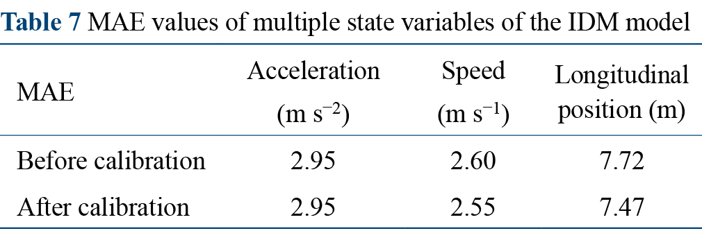
To compare trajectory prediction effects before and after IDM parameter calibration, five pairs of front-rear vehicle data with strong car-following relationships are randomly selected from data excluding parameter calibration for verification of calibration effects. MAE is selected as the evaluation indicator. The MAE calculated from the five subject vehicle acceleration, speed, and longitudinal position prediction results is averaged. The prediction errors before and after IDM model parameter calibration are shown in Table 7, which shows that the prediction results of calibrated IDM model parameters do not differ much from the original IDM model prediction using empirical parameters. Since prediction results do not differ much after parameter calibration, considering that the traffic scenarios from roadside sensing data sources are relatively singular and the amount of roadside sensing data is insufficient, calibration results may not have universality. Therefore, for IDM model parameters, the empirical design values described in section 4.1 are still adopted.

Since the sensing range of roadside sensing equipment is insufficient to cover entire road segments, vehicles can only be recognized as "existing" after entering the sensing range, so the reasonable prediction time interval is the time period when vehicles that actually exhibit stopped queuing behavior enter the roadside sensing range. In selecting prediction time starting points, the prediction time starting point needs to be after the moment when vehicles known to exhibit stopped queuing behavior enter the roadside sensing range, and simultaneously before the moment when the red light cycle turns green.

Figure 9 shows numerical comparisons of true values and model-predicted values of the maximum number of queued vehicles in different lanes at each intersection for the moment when the most recent red light turns green, closest to the collection time, within reasonable prediction time intervals at 1 s time intervals. From top to bottom represent Intersection 2, Intersection 3, and Intersection 4, respectively, where the left and right column figures represent the data distribution of model-predicted values and true values for right lanes and left lanes, respectively, totaling 114 groups of data. True data values are obtained by statistics of the maximum number of queued vehicles cumulatively formed during each red light period.

Figure 9 Comparison of prediction results for maximum number of queued vehicles in different lanes at each intersection

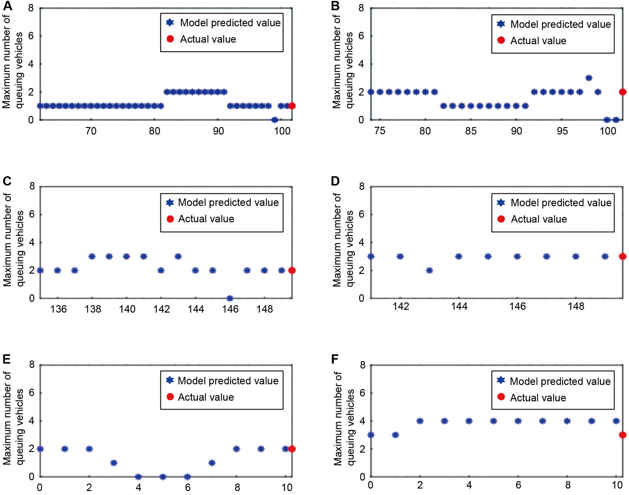
From Figure 9, it can be seen that under most prediction times, the error between model-predicted values and true data values is small. The calculated MAE is 0.4474 and the MAPE is 25.73%. Therefore, the established prediction model can be considered reasonable and can be used to support urban green wave cruise applications under V2I backgrounds. Analyzing Figure 9, model prediction results are based on road traffic state information updated by roadside facilities. When vehicle arrival information tends to stabilize, this method can more accurately predict the maximum number of queued vehicles and queue changes ahead of intersection stop lines during the next red light period, approaching closer to true results. It is also found that vehicles tend to maintain middle lanes rather than rightmost lanes when driving on roads. Due to differences in driver driving behavior and starting/acceleration loss times, certain deviations between true values and model-predicted values are expected.