ContentsFigures & Tables
The application of optical diagnostic technologies in combustion is becoming more extensive, covering areas like the interaction between flow and flame [1], point extinction [2], soot production [3], and combustion instability [4]. Results from these diagnostics are usually obtained in image form. In data acquisition, data gathered by optical measurement systems inevitably includes noise, resulting from inherent sensor noise, optical system defects, and external environmental factors. Therefore, denoising this data to ensure the information's accuracy and extracting subsequent combustion characteristic parameters is a critical step in data processing.
CH-PLIF measurement is a typical application of optical diagnostics in the combustion field. CH is a key component in the combustion chemical reaction process of hydrocarbon fuels, and its position marks the final step of the decomposition of hydrocarbon fuels [5]. Therefore, it reflects the location of the chemical reaction zone and is one of the important markers in optical measurements. CH measurements can obtain the characteristics of the reaction zone under strong turbulence conditions, and the flame front can be extracted [6, 7]. However, under strong turbulence and low equivalence ratio conditions, the concentration of CH radicals is low, and their lifetime is short, resulting in a low signal-to-noise ratio (SNR) in CH measurements [8, 9]. In high-pressure environments or high-frequency measurements, the weak energy of single-pulse lasers further reduces the SNR [10, 11]. Researchers such as Meier et al. [12] captured CH-PLIF distributions in flames with different Reynolds numbers (15 000, 30 000, 45 000, and 58 000) under high turbulence conditions. They found that some experimental images were affected by background noise, presenting a sawtooth pattern. Che et al. [13] investigated the effects of laser wavelength, laser energy, and equivalence ratio on CH-PLIF imaging. The results indicated that CH signals primarily exist at the base of the flame under low equivalence ratio conditions, with weak signal intensity. Furthermore, the excitation of CH signals requires an appropriate laser wavelength and energy; either too high or too low will reduce the SNR of CH-PLIF images. Especially when the equivalence ratio is below 0.7, the significant reduction in SNR makes CH-PLIF measurements quite rare [14]. For small amounts of background noise, methods such as median filtering [15, 16], Gaussian filtering [17, 18], wavelet denoising [19], and combined thresholding methods [20, 21] can effectively remove background noise. These methods perform well when there is a clear distinction between background noise and the signal. However, when processing low SNR images, traditional methods often struggle to precisely distinguish between signal and noise, which may result in noise residue or the inadvertent removal of the signal. Miyauchi et al. [22, 23] conducted simultaneous CH-PLIF, OH-PLIF, and PIV measurements. Their experimental results show that the SNR of CH-PLIF images is significantly lower than that of OH-PLIF images, a phenomenon also observed in other studies [24–26]. Even under low equivalence ratio conditions, the OH signal strength remains relatively high [27]. In some studies, high SNR OH-PLIF images were still captured under low equivalence ratio (<0.6), high pressure, and high turbulence conditions [28, 29]. Furthermore, CH and OH exhibit a certain spatial correlation in the combustion field. For these reasons, we believe that OH-PLIF images can assist in the denoising of CH-PLIF images.
Traditional image denoising methods can be classified based on their principles into spatial domain filtering, transform domain filtering, statistical models, and Hybrid denoising techniques [30]. In practical applications, Gaussian noise and salt-and-pepper noise are the two most common types of noise [31]. Gaussian filtering and median filtering in spatial domain filtering are effective at handling these two types of noise, and are therefore the most widely used in practical applications. With the rapid development of artificial intelligence technologies, neural networks, due to their excellent learning ability, versatility, and flexibility, are playing an increasingly important role in multiple fields. Especially in the field of image denoising, the application of neural networks has significantly surpassed traditional image processing technologies and can effectively handle more complex noise issues. In fields such as medical imaging [32], aerial photography [33], digital photography [34], and industrial inspection [35, 36], the efficient denoising capabilities of neural networks have been widely applied and recognized. Additionally, neural networks have shown their potential in post-processing for optical diagnostics. For example, Hasti and Shin [37] successfully used an improved U-Net network for denoising and droplet reconstruction of spray images; Han et al. [38] used an unsupervised convolutional denoising autoencoder (CDAE) to extract deep image features automatically; Strässle et al. [39] used deep learning methods to extract the flame front from PLIF images; Barwey et al. [40–42] used neural networks to reconstruct the velocity distribution in the flame field from PLIF-OH images.
Given the current issues in PLIF measurements and the outstanding performance of neural networks in image denoising, this paper proposes an innovative denoising strategy. The strategy combines the advantages of U-Net and ResNet networks to construct a novel denoising neural network model. It utilizes the characteristics of OH-PLIF signals, maintaining a high signal-to-noise ratio under low equivalence ratio conditions, along with the synchronous measurement technique with CH-PLIF, to achieve noise removal in CH-PLIF measurements. This method can potentially be extended to the processing of other optical measurement images.
The structure of this paper is as follows: Section 2 introduces the basic concept and architectural details of the denoising model; Section 3 details the experimental design and data processing strategies; Section 4 describes the model's training process and compares its performance with other denoising models; and Section 5 provides a detailed summary of the research findings.
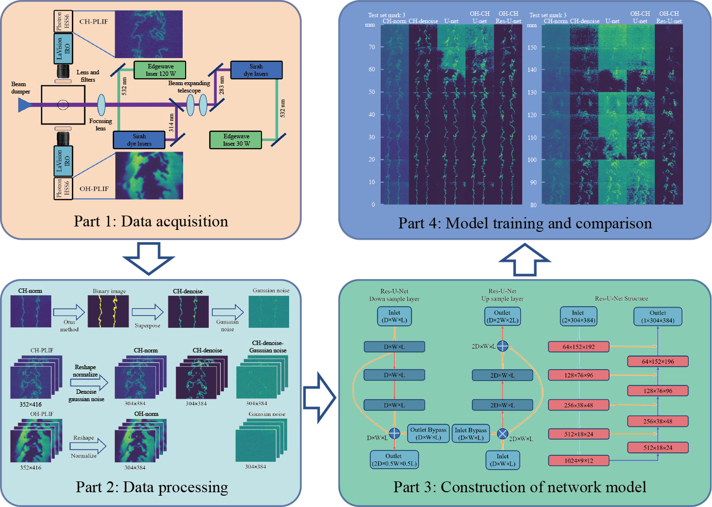
Figure 1 shows the workflow for building the denoising model proposed in this research, segmented into four crucial steps: data acquisition, data processing, construction of network model, and model testing and comparison.
Data acquisition: Through a CH-OH-PLIF high-speed measurement system, images of CH and OH distributions are captured at various positions above the outlet of the experimental combustor and are categorically stored based on different operational conditions.
Data processing: The collected image data is preprocessed, including normalization to the range of 0–1, followed by denoising, data fusion (Concat), and the addition of Gaussian noise based on the normalized data.
Construction of network model: Constructs a Res-U-Net network, employing the preprocessed data to build and train the network model.
Model testing and comparison: Data that has never been encountered is input into the network to test the model's generalization ability and compare its performance with other existing models, thereby validating the proposed model's superiority.
Neural network types include fully connected neural networks, convolutional neural networks, recurrent neural networks, generative adversarial networks, and Transformer networks. Each has its own advantages, and the most suitable network architecture should be selected based on the specific application scenario. For image data, convolutional neural networks can capture spatial structural information while maintaining spatial invariance. Additionally, the use of convolution operations significantly reduces the computational load.
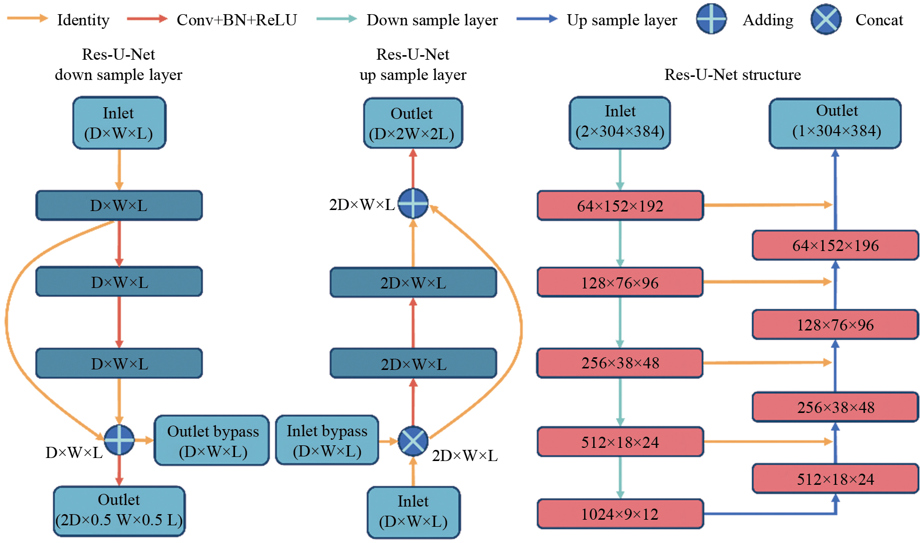
Two important network architectures emerged in developing convolutional neural networks: ResNet [43] and U-Net [44]. Before the advent of ResNet, it was observed that increasing the number of layers in convolutional neural networks (CNNs) for hierarchical learning could effectively enhance the network's ability to learn high-level features of images, thereby improving its expressive power. However, as the number of layers increases, it becomes difficult for errors to be effectively backpropagated to all layers during the learning process, leading to vanishing and exploding gradients [45], limiting the development of deep CNNs ResNet introduced the idea of residual learning into the CNN domain, using direct connections between different layers to allow the network to skip unnecessary learning processes, effectively solving the gradient explosion problem caused by increased network depth. The U-Net model is an improvement on fully convolutional networks (FCN) [46], featuring a symmetric encoder-decoder architecture and using skip connections to link different layers of the encoder and decoder. This enables the extraction of different levels of features from the image while preserving the spatial information, thereby achieving pixel-level classification.
This study proposes a novel network architecture that combines the advantages of U-Net and ResNet, called Res-U-Net, with its structural details shown in Fig. 2. Res-U-Net retains the encoder-decoder framework of U-Net, but introduces the residual connection concept of ResNet in the downsampling and upsampling layers of both the encoder and decoder parts, to enhance the model's ability to capture relevant information and reduce interference from irrelevant information.
In the training process of common denoising models, the model first receives noisy images, which are typically simulated by adding Gaussian noise, salt-and-pepper noise, or Poisson noise to the original clear images. Then, the model processes these noisy images and outputs the denoised images. Next, the model compares the denoised image with its original clear image, and calculates the loss function by analyzing the differences between the two. The value of this loss function is used to guide the optimization process of the denoising model, with the goal of minimizing the difference between the denoised image and the original clear image, thereby improving the denoising performance of the model.
This method effectively solves most denoising problems and has become the mainstream strategy for addressing this challenge. However, when measuring CH radicals in flames, we encounter two major challenges: the naturally low concentration and short lifetime of CH radicals. Particularly, when high-frequency shooting is employed, the energy released by each laser pulse is relatively low, which further reduces the fluorescence signal strength of CH radicals, leading to a significant decrease in the SNR of the CH images, thereby affecting the effectiveness of this method.
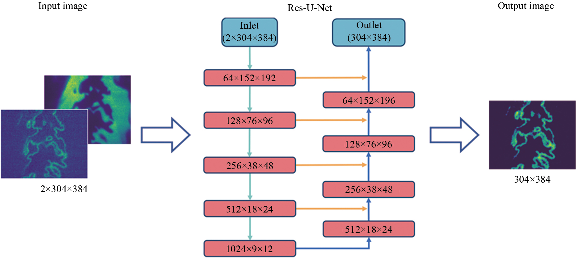
In hydrocarbon fuel flame environments, OH radicals usually have a higher concentration in the high-temperature products of the flame, and many studies have confirmed that the spatial distributions of OH and CH radicals exhibit a certain degree of overlap [47–49]. Based on this characteristic, our study attempts to input both the CH images to be denoised and the OH images simultaneously into the Res-U-Net network, utilizing the information from the OH images to assist in the denoising process of the CH images. This denoising method is referred to as CH-OH cooperative denoising, with the specific process shown in Fig. 3. This method leverages the correlation between the two radicals, providing a new perspective and support for the denoising of CH images, with the aim of improving the denoising performance through this cooperative processing approach.
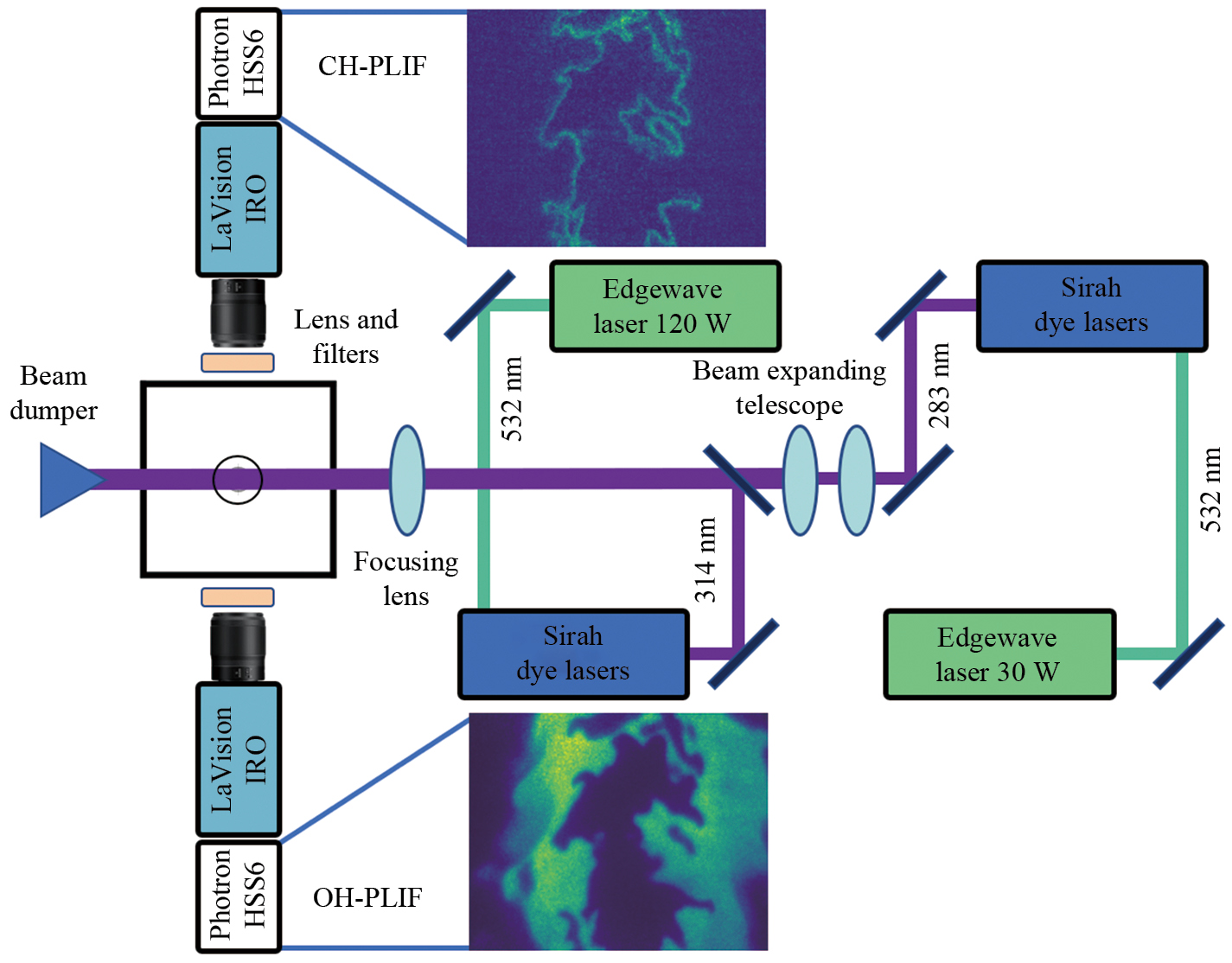
The experiments in this study were mainly conducted at the Clean Combustion Laboratory at the University of Sydney, utilizing a high-speed CH-OH-PLIF imaging system, as shown in Fig. 4. The system includes two laser diagnostic devices for OH-PLIF and CH-PLIF, as well as a burner. The burner has adjustable equivalence ratio (Φ), volumetric flow rate (V), flow split ratio (Q), and the distance between the measurement point and the burner exit (d). The turbulent Reynolds number (Ret) of the flame is controlled by adjusting V and Q. For more structural details, refer to Ref. [50]. In the CH-PLIF system, a 120 W EdgeWave laser generates a 532 nm laser at a frequency of 10 kHz, which pumps a Sirah dye laser to generate a 632 nm laser. The laser is frequency-doubled to generate 315.589 nm ultraviolet light. Then, a sheet beam optical element is used to expand the ultraviolet light to a width of 40 mm in the vertical direction and focus it directly above the burner exit, to excite the C-X electronic transition of CH molecules in the flame. For the OH-PLIF system, a 30 W EdgeWave laser generates a 532 nm laser at 10 kHz, which also pumps a Sirah dye laser to generate a 566 nm laser. Through frequency doubling and separation, 283.553 nm ultraviolet light is generated, and this beam is expanded to a width of 40 mm in the vertical direction by a sheet beam optical element and also focused directly above the burner exit, to excite the A-X electronic transition of OH molecules in the flame.
The fluorescence signal collection system consists of two couple-charged device (CCD) cameras equipped with amplifiers. To reduce interference from Rayleigh scattering at a wavelength of 283 nm, the camera collecting OH fluorescence signals is fitted with a 315 nm ±10 nm bandpass filter, specifically designed to capture the desired fluorescence signals. Meanwhile, the camera collecting CH fluorescence signals uses a 300 nm long-pass filter to collect the relevant fluorescence signals. To avoid interference from Rayleigh scattering signals at 315 nm, the OH excitation beam is delayed by 250 ns compared to the CH excitation beam. The fields of view (FOV) for the OH and CH signal collection are the same, measuring 24 mm × 28 mm. This setup ensures that the fluorescence collection system accurately captures the required fluorescence signals while minimizing interference and improving the quality and reliability of the experimental data.
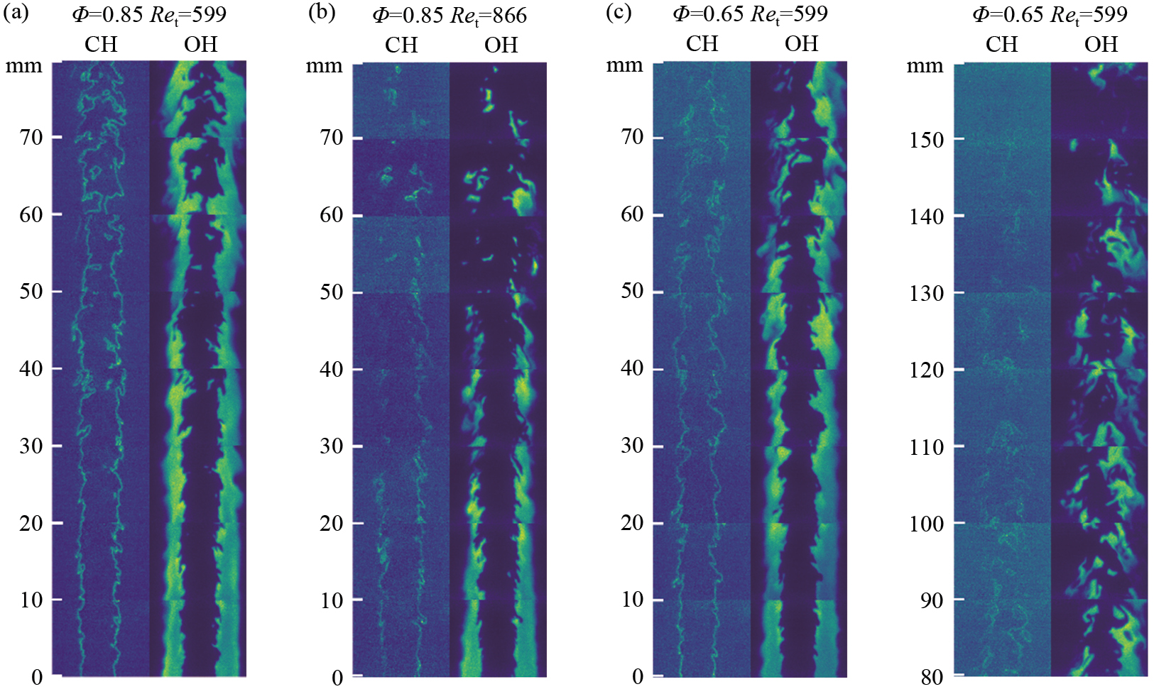
Figure 5 shows CH-OH-PLIF images under different equivalence ratios (Φ=0.65, 0.85) and turbulent Reynolds numbers (Ret=599, 866). In Fig. 5 (a), images obtained under Φ=0.85 and Ret =599 conditions are displayed, where both OH and CH images are relatively clear. It can be observed that as the capturing height increases, the flame front begins to exhibit a distortion phenomenon. Nevertheless, the signal-to-noise ratio (SNR) of the CH image remains high, allowing for clear identification of the CH radical distribution. Comparing Fig. 5 (a) with Fig. 5 (b), it can be seen that an increase in the volumetric flow rate raises the turbulence level of the airflow, causing the flame front to rapidly break up at higher capturing heights, with a corresponding decrease in the CH radical SNR. Comparing Fig. 5 (a) with Fig. 5 (c), when the equivalence ratio is reduced to Φ=0.65 under Ret=599 conditions, the already low CH radical fluorescence signal is further weakened due to the reduction in equivalence ratio, particularly at higher capturing heights, where the CH image's SNR significantly decreases.
Typically, to address the problem of denoising, the construction of a dataset begins with acquiring high-quality, clear original images, upon which noise is artificially added to simulate low signal-to-noise ratio conditions. This aims to create a pair of images: one being the clear original, and the other being the noise-added image. This pair of images is then used to train the denoising network. However, in this study, the CH images obtained inherently contain a certain degree of noise, with no completely noise-free images available. Therefore, we must preprocess the existing images to ensure they meet the requirements for training the denoising model.
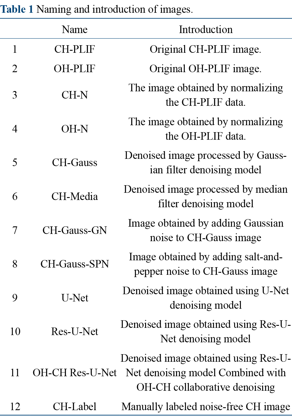
For clarity, the images mentioned in this paper are labeled and briefly described in Table 1.
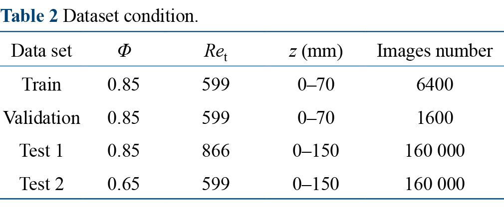
Low-noise images are required as label images for the training process when constructing the model. As shown in Fig. 5, under the conditions of Φ=0.85 and Ret=599, the fluorescence signal of the CH radical is significantly stronger, resulting in a higher image signal-to-noise ratio. In this case, the distinction between the CH signal and noise in the image is quite clear (the average signal-to-noise ratio of the CH-Norm image exceeds 15 dB under this condition). Separating CH signal and noise is relatively easy, and the data is divided into training and validation sets with an 8:2 ratio. Meanwhile, the other two conditions shown in Fig. 5, Φ=0.85, Ret=866, and Φ=0.65, Ret=599, are used as test sets, aiming to evaluate the model's denoising performance under higher turbulence and lower equivalence ratio conditions. The specific division of conditions is shown in Table 2.
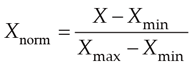
Given the significant difference in fluorescence signal intensity between CH and OH, the pixel values of the two in the original image are vastly different. To reduce the dependency between features and enhance the model's generalization ability, we normalized the pixel values of the CH and OH images to the range of 0 to 1 using the normalization Eq. (2). The normalized images are then named CH-N and OH-N, respectively.(1)
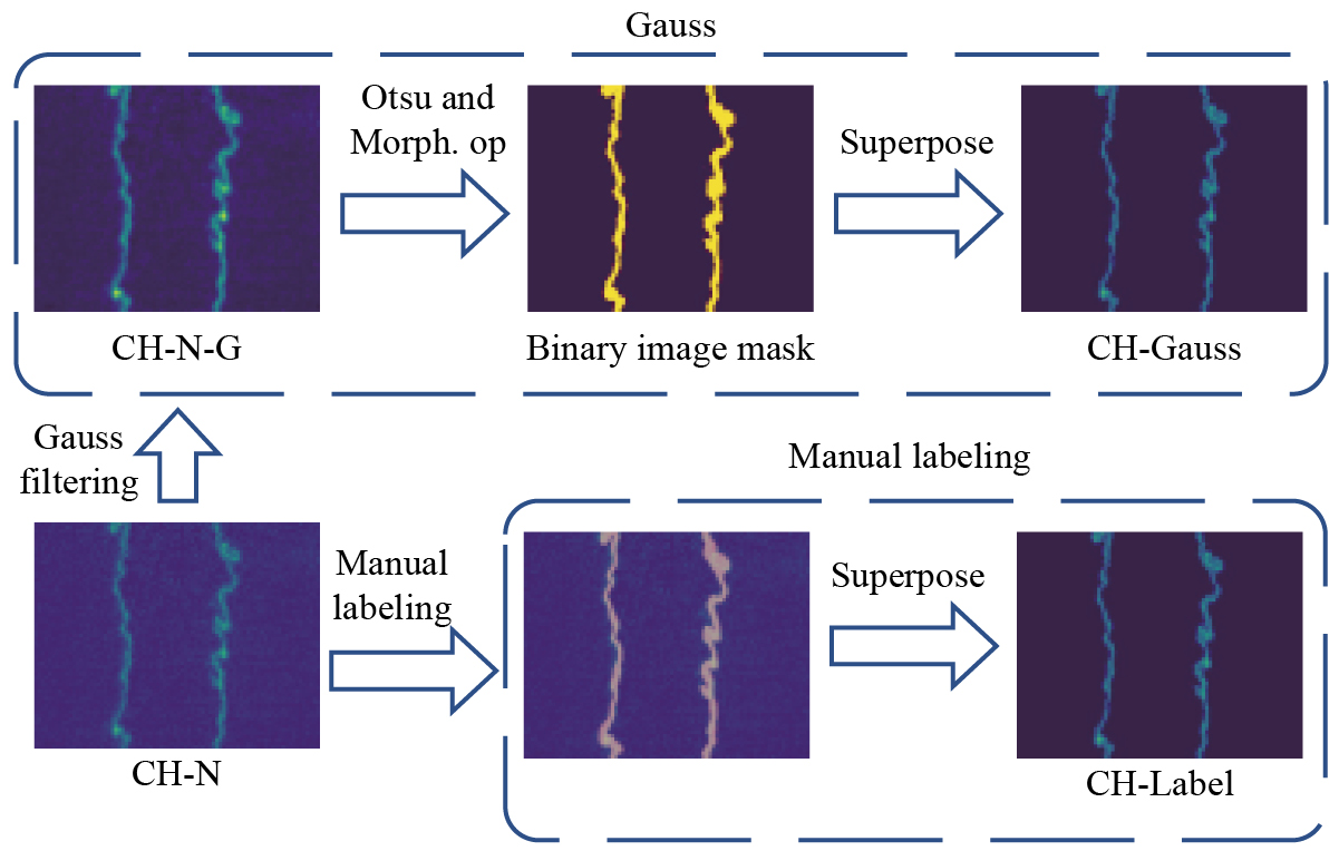
After normalizing the dataset, the training dataset is extracted separately, and Gaussian filtering is applied to the CH-N images (denoted as CH-N-G). Gaussian filtering aims to remove high-frequency noise in the image, thereby reducing its complexity. Then, the Otsu method calculates the threshold for the CH-N-G image to maximize the weighted value of the squared difference between the pixel intensity and its average intensity, generating the binary image mask. To further optimize, morphological operations are used to remove small noise points in the binary image, and the processed CH-N-G is overlaid with the binary image mask, achieving binary segmentation and effective noise reduction of the CH-PLIF image. This process is illustrated in Fig. 6. For convenience, this noise reduction method is referred to as "Gauss", and the resulting image is named CH-Gauss, which will serve as the reference image for the model output. The method where Gaussian filtering is replaced by median filtering is referred to as "Media", and the resulting image is named CH-Media.
To better evaluate the denoising effect of different models, the open-source data annotation tool Label-Studio is used to manually label a portion of the original images in the validation set. For each height (z), 100 images are taken, resulting in a total of 8×100=800 images, forming the noise-free dataset CH-Label. The specific process is shown in Fig. 6.
As shown in Fig. 3 above, the Res-U-Net model is trained on the training set using the CH-OH collaborative denoising method. During the training process, each round of input consists of two images: one is OH-N, and the other is the corresponding CH-N image (OH-N & CH-N). Models using the CH-OH collaborative denoising method are distinguished by the prefix "CH-OH" added to their names. The model calculates the loss value (Loss) by comparing its predicted output with the corresponding CH-Gauss image, and updates the model's neuron coefficients based on this loss value.
The training configuration includes a batch size of 10, with all model parameters optimized using the Adaptive moment estimation (Adam) optimizer and an initial learning rate set to 1e–3. The loss function used is mean squared error (MSE), and these hyperparameters were selected based on repeated experimental validation to determine the optimal configuration. All the code is written using the Pytorch framework and leverages compute unified devices architecture (CUDA) technology for accelerated computation. The computer configuration used for model training is: Intel® Xeon® Silver 4210R CPU * 2, NVIDIA GeForce RTX 2080Ti 11G GPU, 64 GB RAM.
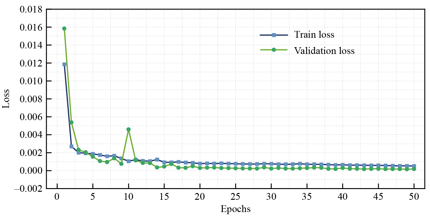
The maximum number of training epochs was set to 50, and we observed significant changes in the loss on both the training and validation sets as the epochs progressed, as shown in Fig. 7. In the early stages of training, specifically within the first three epochs, the loss on the training set decreased sharply. Subsequently, from epoch 3 to epoch 15, the loss reduction rate significantly slowed down. After that, although the loss decreased, the reduction was extremely limited. On the other hand, the loss on the validation set decreased rapidly during the first six epochs, followed by some fluctuations between epochs 6 and 20, though the overall trend remained downward. This may be attributed to the training process becoming trapped in a local optimum, which caused the optimization direction to deviate from the global optimum, but in a subsequent epoch, the model escaped this local region and moved into a more favorable optimization region. After that, the loss reduction rate became very slow and almost stabilized. The training result at the end of epoch 50 was selected as the final form of the model.
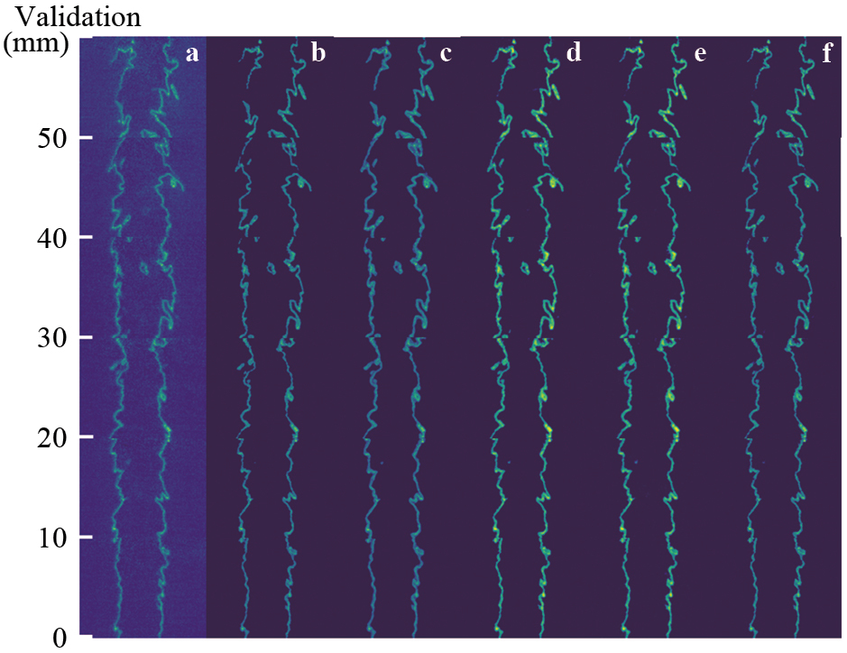
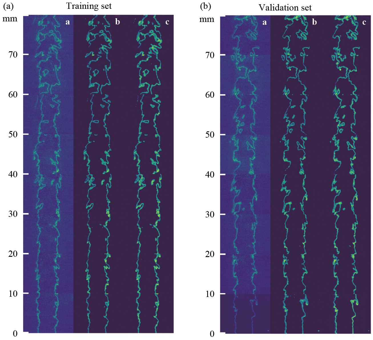
The Res-U-Net model using the CH-OH collaborative denoising strategy performs excellently in extracting CH signals in both the training and validation sets, and when compared to the Gauss method, both show high consistency. Specific results are shown in Appendix Fig. A1. This study compares traditional denoising methods with other commonly used neural network denoising models. The traditional denoising methods include the Gauss model and Media model introduced in Section 2.2.2, while the neural network methods include the U-Net model and Res-U-Net model. Figure 8 shows the denoising performance of different models on the validation set, where the denoising effects of the Gauss model, Media model, and OH-CH Res-U-Net model are closest and yield the best results. Although the U-Net model and Res-U-Net model also effectively reduce noise in the images, these two models tend to enhance the CH signal strength.
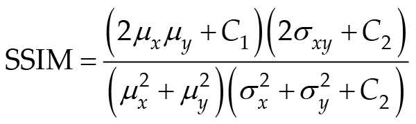
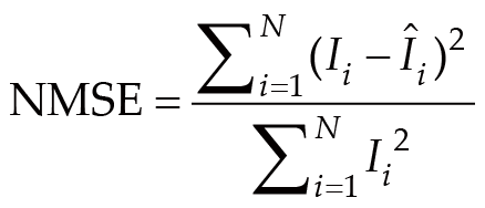
In the field of image denoising, peak signal-to-noise ratio (PSNR), structural similarity index (SSIM), and normalized mean squared error (NMSE) are three commonly used metrics to evaluate the quality of image denoising. PSNR assesses the image restoration quality by comparing the pixel differences between the original and processed images. Its value is measured in decibels (dB), with higher values indicating better denoising performance. SSIM is a metric for evaluating the similarity between two images, taking into account image luminance, contrast, and structural information. The SSIM value ranges from −1 to 1, with values closer to 1 indicating that the denoised image is more similar to the original image. NMSE directly compares the pixel value differences between images, providing a unified standard across different scales or image backgrounds, with smaller values indicating greater similarity.
The formulas for the three metrics are as follows:(2)(3)(4)
MSE stands for mean squared error, which is used to evaluate the error between CH-Denoise images and the denoised images from various models; MAXⅠ refers to the maximum energy peak of the signal; bits represent the bit depth of pixel values in a single channel of the image; μ and σ respectively represent the mean and variance of the image; σxy is the covariance between image x and image y; C1 and C2 are small constants used to stabilize the division operation, typically set to 0; Ii is the i-th pixel value of the original image, is the i-th pixel value of the denoised image, and N is the total number of pixels in the image.
Table 3 presents the performance metrics of different models on the validation set. The PSNR, SSIM, and NMSE for each image were calculated by comparing with the CH-Label and then averaged. This is consistent with the direct comparison of image results, where the Gauss, Media, and OH-CH Res-U-Net models demonstrate the best denoising performance.
Gaussian noise follows a Gaussian distribution (also known as a normal distribution) and simulates random noise in images, similar to the noise caused by the random performance of electronic devices. Salt-and-pepper noise appears as random black-and-white pixels in an image, simulating the sporadic noise that may occur during image acquisition or transmission, akin to sudden anomalies. These two types of noise are common artificial noises used to test the performance of denoising models [51, 52].
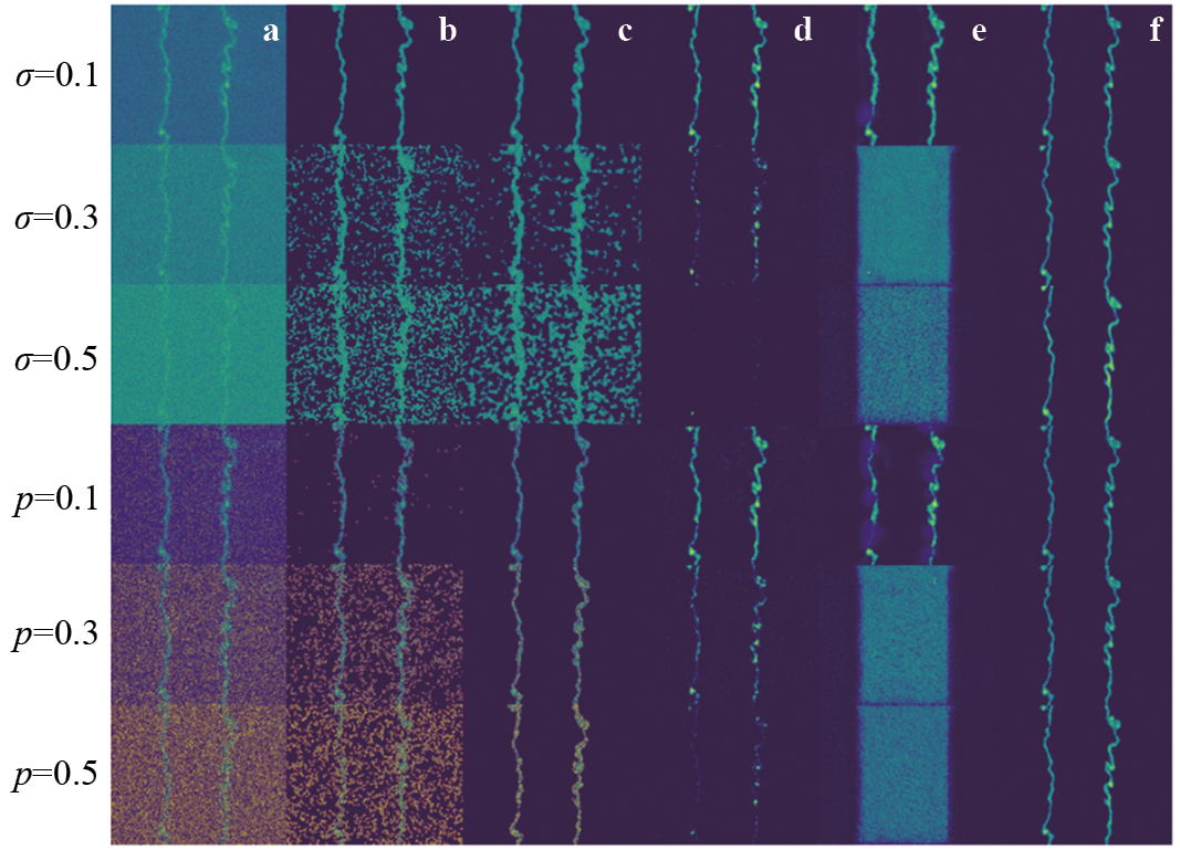
Artificial noise of different intensities was added to the CH-Gauss images to evaluate the performance of different models systematically in handling noise of varying intensity and types. The results are shown in Fig. 9, where column (a) displays the CH-N images with different intensities of noise added. The first three rows add Gaussian noise, with the intensity controlled by adjusting the variance σ. The last three rows have salt-and-pepper noise added, with the intensity controlled by adjusting the noise density p. Columns (b) to (f) show the denoising effects of different models on these six images.
The Gauss model shows significant denoising performance when handling Gaussian noise with a standard deviation of σ=0.1 and salt-and-pepper noise with a noise density of p=0.1. However, as σ and p increase, its denoising performance significantly decreases. The Median model performs similarly to the Gauss model when handling Gaussian noise, with better denoising results at σ=0.1, but its performance deteriorates sharply as σ increases. In contrast, the Median model has a significant advantage in handling salt-and-pepper noise, effectively distinguishing noise, but as p increases, the CH signal is significantly enhanced. The U-Net model performs well under noise conditions of σ=0.1 and p=0.1, effectively separating CH signals from noise and filtering out the noise. However, as noise intensity increases, the model's ability to distinguish CH signals significantly decreases, especially under conditions of σ=0.5 and p=0.5, where a large amount of CH signal is misclassified as noise. The Res-U-Net model performs relatively well under noise conditions of σ=0.1 and p=0.1, but there are still instances where some CH signals are misclassified as noise. As noise intensity increases, the performance of this model gradually weakens, and may even have adverse effects. In contrast, the OH-CH Res-U-Net model demonstrates excellent denoising capabilities across various noise intensities and types. Although it may enhance the CH signal under high noise intensity conditions, its ability to restore the distribution of CH signals remains superior.
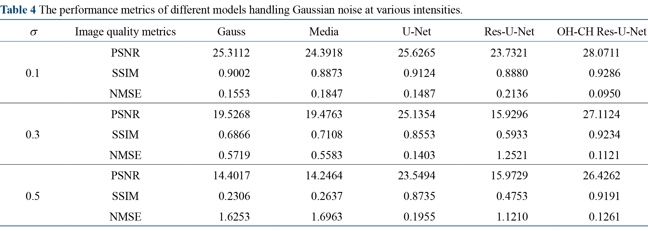
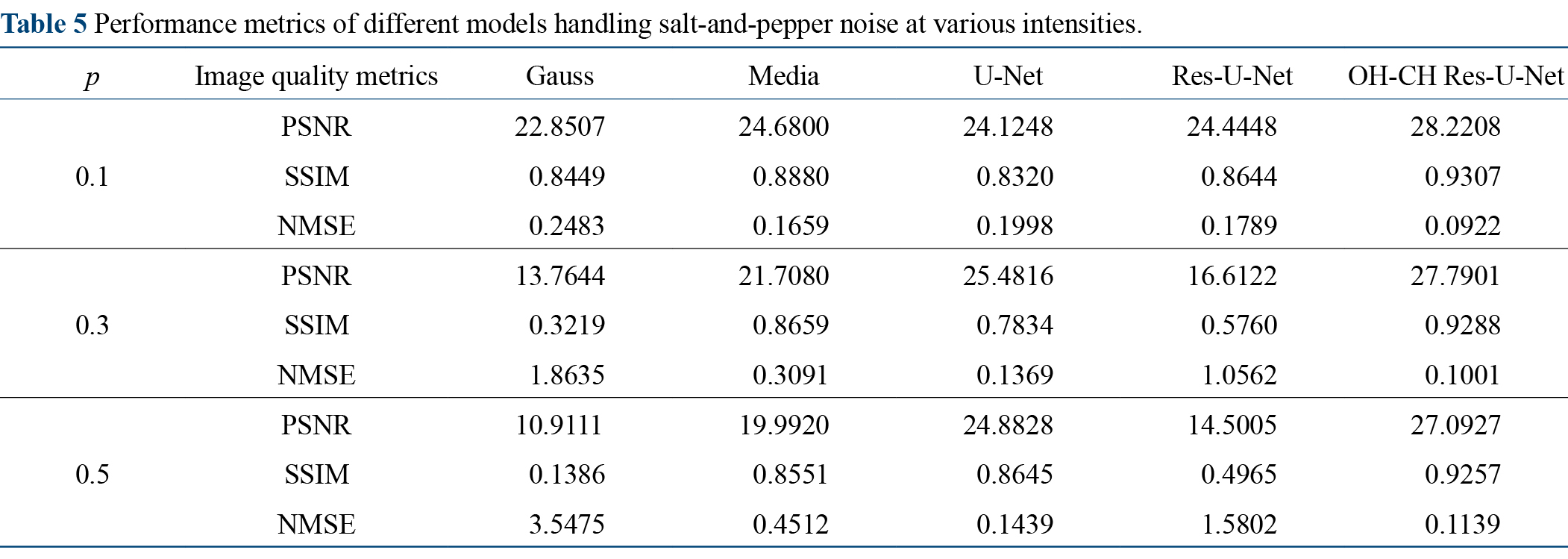
Tables 4 and 5 present the performance metrics of different models in handling Gaussian noise and salt-and-pepper noise at different intensities. The Gauss model and Media model show similar performance when handling Gaussian noise. As the intensity of Gaussian noise increases, the denoising performance of the models deteriorates. This is because the denoising principles of these two models heavily rely on pixel intensity. When the noise signal intensity increases, it becomes difficult to distinguish the CH signal. The Media model performs better when handling salt-and-pepper noise. However, a significant portion of the noise overlapping with the CH signal is retained. The U-Net model shows consistent performance in handling Gaussian noise and salt-and-pepper noise at different intensities. The performance metrics decrease as the noise intensity increases. For the Res-U-Net model, the performance metrics decrease significantly as noise intensity rises. Among all models, the OH-CH Res-U-Net model shows the best performance metrics. As the intensity of artificial noise increases, the decrease in performance metrics is relatively small.
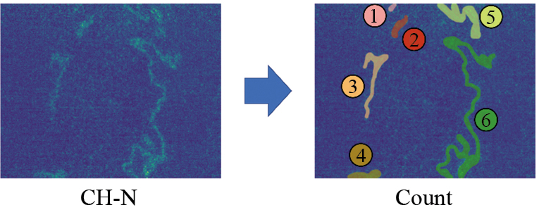
Due to the low signal-to-noise ratio of the test set data, it is difficult to obtain "noise-free" images, making it impossible to evaluate the denoising performance of the model by calculating PSNR, SSIM, and NMSE. Therefore, in this study, manual annotation was performed on a subset of CH-N images from the Test 1 and Test 2 datasets (50 images randomly selected from each height z, totaling 32×50=600 images), as shown in Fig. 10. The average number and area of CH segments in CH-N images at each height were calculated, with the area represented by the number of pixels.
Due to the large number of denoised images processed by different models (600×5=3000 images), manual annotation would be time-consuming, and the statistical results may vary due to differences in annotators' standards. Since the images processed by the models have an improved signal-to-noise ratio compared to CH-N images, the Otsu method can be used to calculate a threshold, generate binary images, and calculate the number and area of CH segments (as shown in Fig. 11). Subsequently, under different height conditions, the average number and area of CH segments in the denoised images of each model are calculated. Since all models use the same method, the consistency of the statistical criteria is ensured. The figure demonstrates the process of counting CH fragments for a Test 2 dataset image using OH-CH Res-U-Net and Res-U-Net. The statistical results of OH-CH Res-U-Net are consistent with the manual annotation results in Fig. 10, whereas the processing by Res-U-Net caused excessive fragmentation of CH fragments, resulting in a significantly higher count than the manual annotation results.
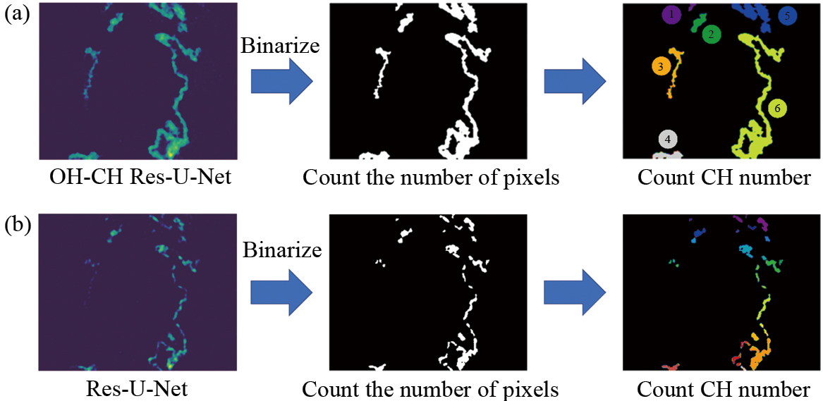
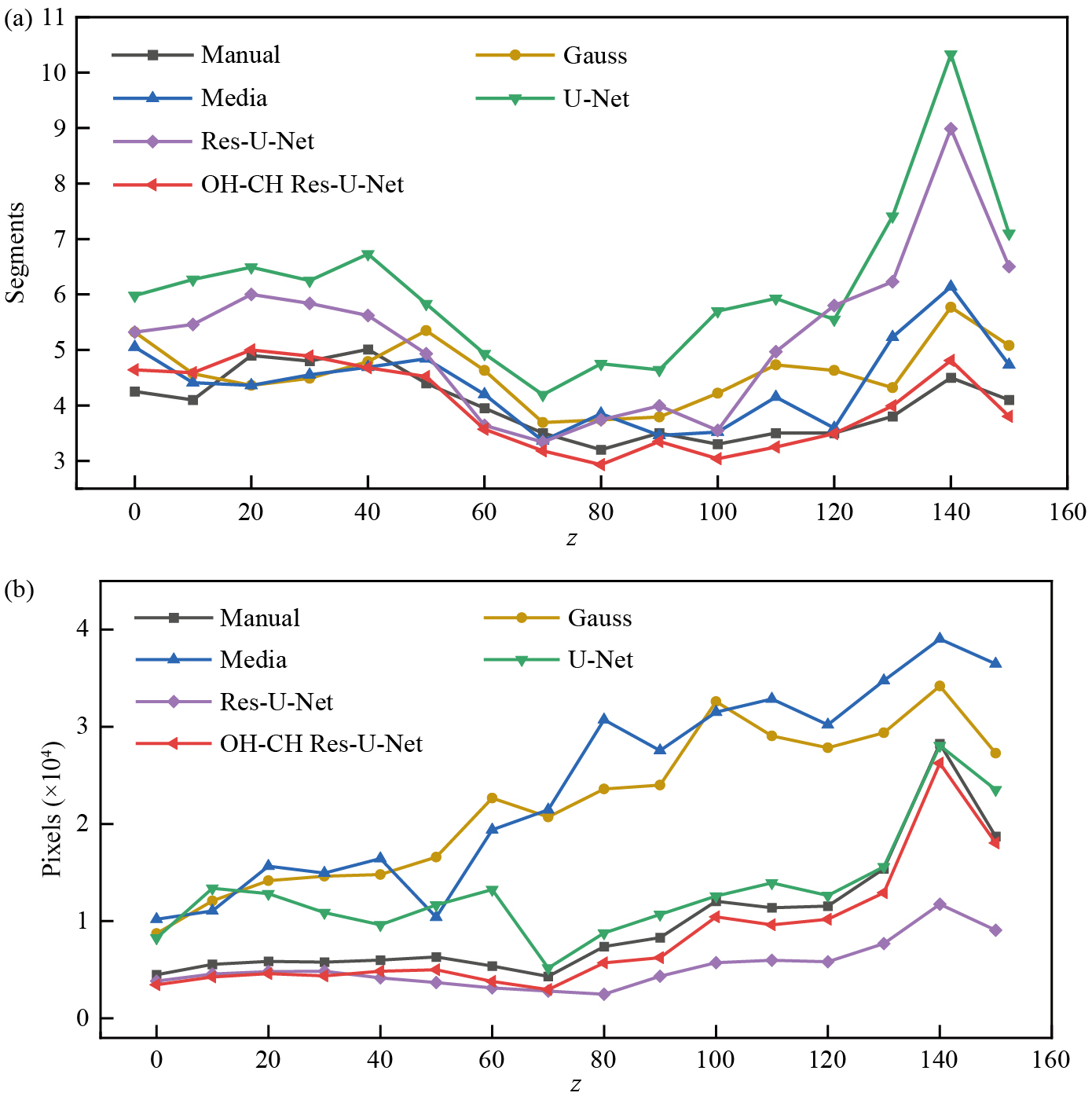
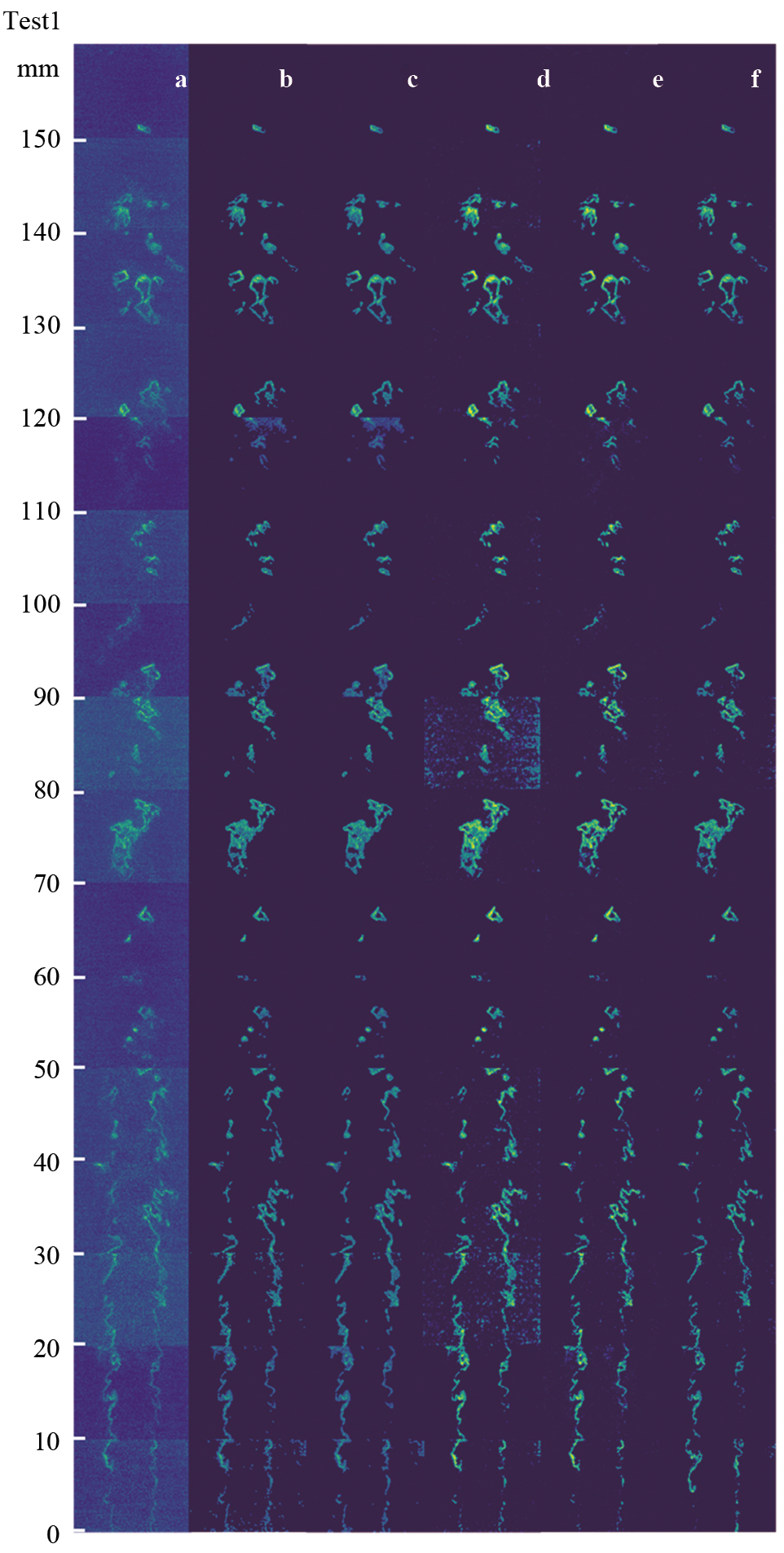
Figure 12 (a) presents the average number of CH segments in images at different heights after denoising by various models under high Ret conditions (Test 1 dataset). At lower imaging heights (small z), the statistical results of the Gauss, Res-U-Net, and OH-CH Res-U-Net models are relatively close to the manual annotations. However, as the imaging height z increases, the error in the number of CH segments identified by the U-Net and Res-U-Net models gradually increases. In contrast, the variation trends of the Gauss, Media, and OH-CH Res-U-Net models are highly consistent with the manual annotations. Among them, the OH-CH Res-U-Net model yields results that are closest to the manual annotations at greater heights (larger z). Figure 12 (b) shows the average pixel area of CH segments at different heights after denoising by various models. At lower image capture heights (z<70), the results of the Res-U-Net and OH-CH Res-U-Net models are very close to the manually processed results. However, as the image capture height increases, the results of the Res-U-Net model gradually deviate from the manually processed results. Meanwhile, the performance of the U-Net model gradually improves, achieving results comparable to the OH-CH Res-U-Net model. Additionally, the results of the Gauss and Media models exceed the manually processed results at all image capture heights. In summary, when processing data under high Ret conditions, the OH-CH Res-U-Net model demonstrates the best overall performance. Appendix Fig. A2 presents the denoising results of different models under high Ret conditions (Test 1 dataset).
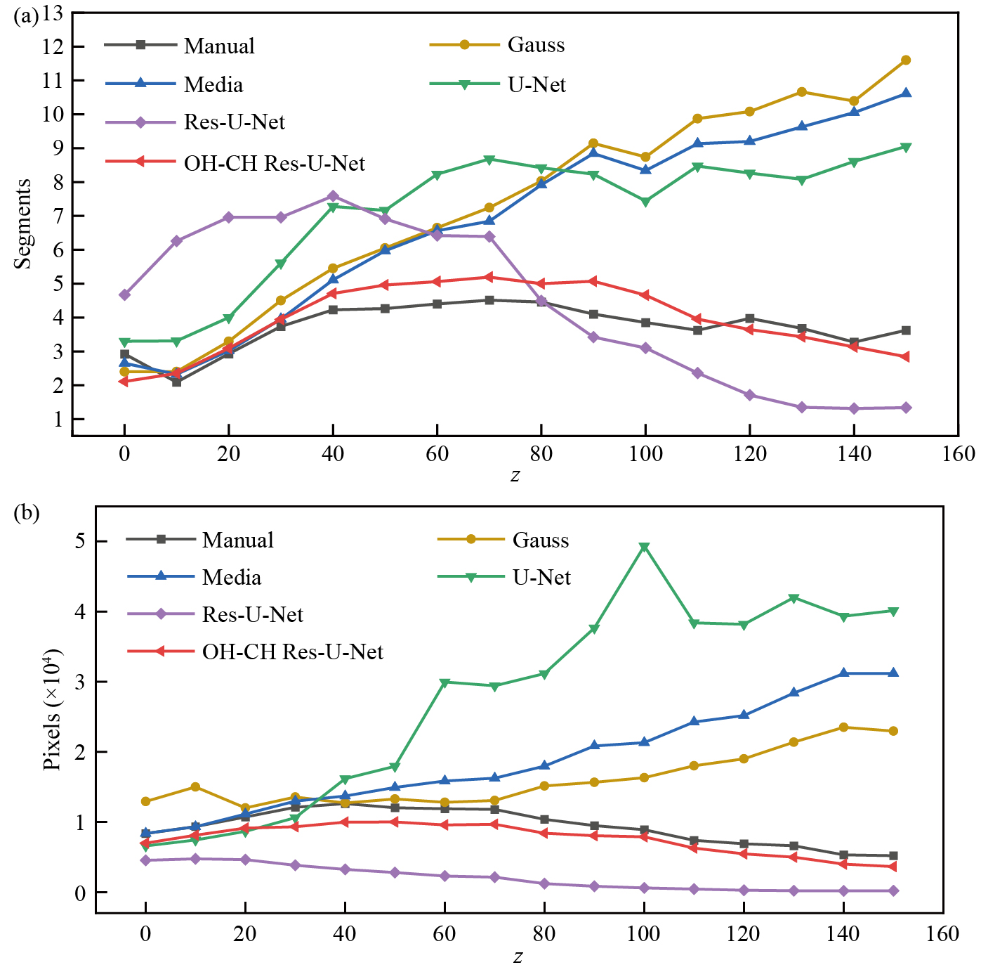
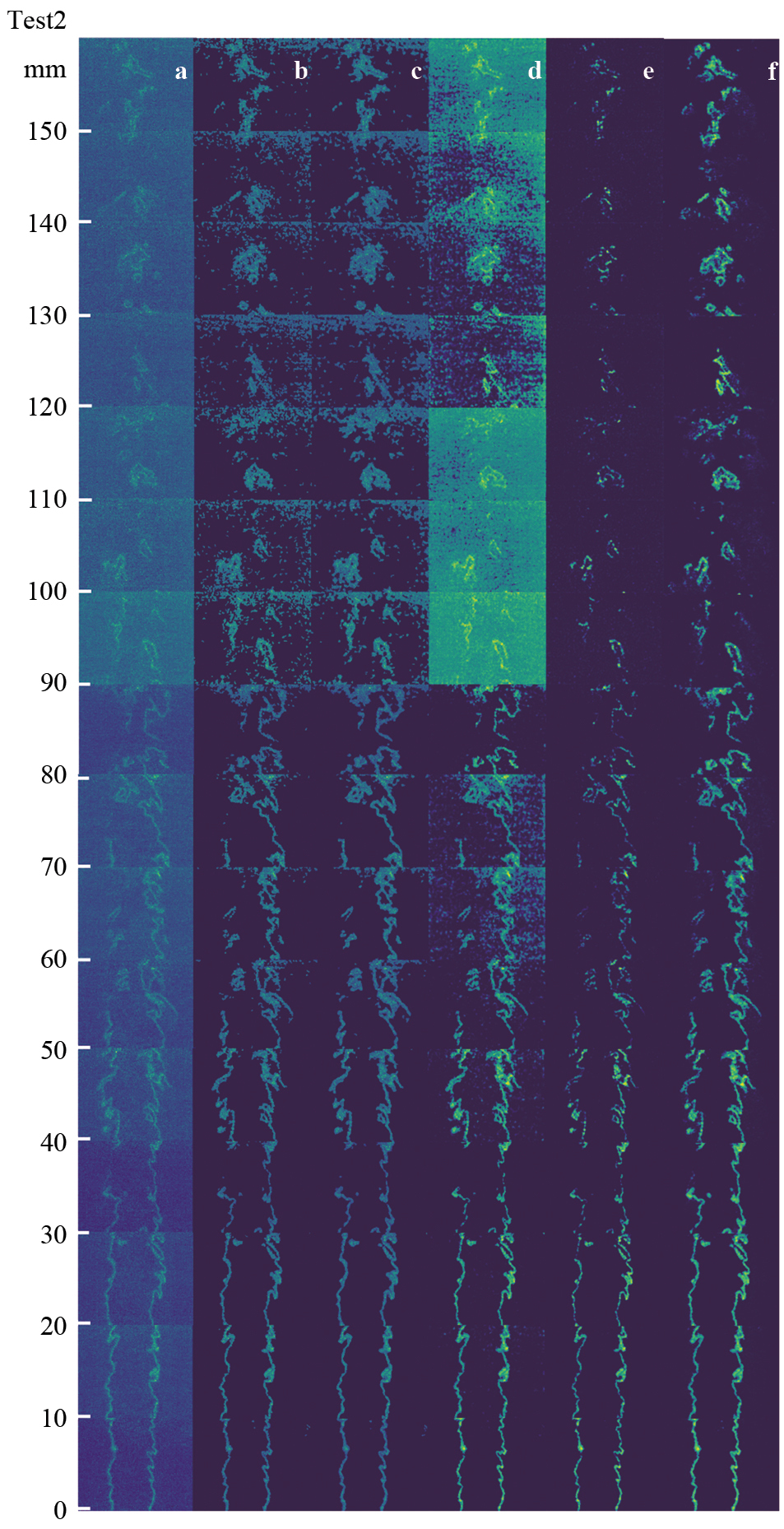
Due to the short lifetime of CH radicals, reducing the equivalence ratio causes a rapid decline in the signal-to-noise ratio of CH-PLIF images. Particularly in images captured at higher heights (large z values), a large amount of noise signals with intensities similar to the CH signal appear, significantly increasing the difficulty of denoising. Figure 13 (a) presents the average number of CH segments in images at different heights after denoising by various models under low equivalence ratio conditions (Test 2 dataset). As the image capture height z increases, the discrepancies between the statistical results of the Gauss, Media, and U-Net models and the manually labeled results gradually increase. In contrast, the statistical results of the Res-U-Net model show an initial increase followed by a decrease, with the CH segment count falling below the manually labeled results when z exceeds 80. Among them, the OH-CH Res-U-Net model demonstrates the best performance. Although there is a slight increase in the discrepancy between the CH segment count from the model and the manually labeled results at lower image capture heights, the overall trend remains consistent. When the image capture height z exceeds 100, the error remains low. Figure 13 (b) presents the average pixel count of CH segment areas in images at different heights after denoising by various models. At lower image capture heights (z<70), the results of the Gauss, Media, and OH-CH Res-U-Net models are very close to the manually processed results. As the image capture height z increases, the Gauss, Media, and U-Net models retain noise, leading to CH area values gradually exceeding the manually processed results. In contrast, the Res-U-Net model exhibits over-denoising, mistakenly removing portions of the CH signal, causing the calculated CH area to be lower than the manually processed results. In summary, under reduced equivalence ratio conditions, the OH-CH Res-U-Net model still outperforms the other models. Appendix Fig. A3 presents the denoising results of different models under low equivalence ratio conditions.
This study proposes a novel optical diagnostic image denoising method, called the Res-U-Net model, which combines the advantages of U-Net and ResNet. To address the situation of extremely low signal-to-noise ratios, the model employs the CH-OH collaborative denoising strategy, designed explicitly for denoising CH-PLIF images, effectively solving the issues of CH signal misdeletion and the introduction of secondary noise. The following conclusions are drawn by comparing the performance of different denoising models on data collected under various parameters:
(1) On the validation set, the denoising effects of the five models—Gauss, Media, U-Net, Res-U-Net, and OH-CH Res-U-Net—are all significant, with clearer CH contours. The U-Net and Res-U-Net models slightly enhanced the CH signal. After comparing with the manually annotated noise-free dataset CH-Label and calculating the PSNR, SSIM, and NMSE metrics, it was found that the Gauss and OH-CH Res-U-Net models performed the best, while the performance of the other three models slightly decreased.
(2) The OH-CH Res-U-Net model still maintains good denoising performance when handling Gaussian noise and salt-and-pepper noise of varying intensities. By comparing the performance metrics of different models, it was observed that the PSNR, SSIM, and NMSE metrics of all models decreased as the noise intensity increased, with the OH-CH Res-U-Net model exhibiting the smallest reduction in performance among all models.
(3) The OH-CH Res-U-Net model still outperforms all other denoising models on the high turbulence Reynolds number dataset (Test 1) and low equivalence ratio dataset (Test 2). The OH-CH collaborative denoising method optimizes the performance of the Res-U-Net network on low SNR images, minimizing the misdeletion of CH signals to the greatest extent.
In summary, under conditions of relatively high equivalence ratio, all types of models can effectively identify and remove noise signals from the images; thus, any model can achieve satisfactory denoising performance under such conditions. Considering the experimental cost, it is not necessary to synchronously acquire CH-OH-PLIF images in such cases. However, when the equivalence ratio decreases and turbulence intensity increases, the signal-to-noise ratio of the images drops significantly, and model performance also deteriorates considerably. Therefore, in such scenarios, it is recommended to use the CH-OH Collaborative Denoising approach, specifically the CH-OH Res-U-Net model, for image processing.
Wei Pan: Writing, validation, coding; Wu Jin: Conceptualization, methodology, diagnostic, supervision; Xiafei Li: Data management, graphic; Qian Yao: Writing, reviewing & editing; Chaowei Tang: Software; Li Yuan: Visualization; Jianzhong Li: Funding acquisition, project administration, supervision.
This work was supported by the National Natural Science Foundation of China (No. 52276118). The authors also wish to express their gratitude to Assaad Masri, Mrinal Juddoo, and Scott A. Steinmetz at the University of Sydney for their support in the experimental implementation.
This paper proposes an innovative denoising strategy to address the issues in current PLIF measurements and leverages the outstanding performance of neural networks in image denoising. A novel denoising neural network model, Res-U-Net, is developed by combining the advantages of U-Net and ResNet. By exploiting the high signal-to-noise ratio characteristics of OH-PLIF signals under low equivalence ratio conditions and their synchronous measurement technique with CH-PLIF, noise removal in CH-PLIF measurements is achieved. This method is expected to be extended to processing other optical measurement images.
C
Channels
z
Height
W
Width
Φ
Equivalence ratio
V
Volume flow rate
Q
Diversion fraction
d
Distance between the shooting point and the combustor exit
Ret
Turbulent Reynolds number
σ
Noise density, adjusting salt-and-pepper noise intensity
p
Noise density, adjusting the intensity of salt-and-pepper noise
A. Alwafi, T. Nguyen, Y. Hassan, and N. K. Anand, "Experimental analysis of a non-isothermal confined impinging single plume using time-resolved particle image velocimetry and planar laser induced fluorescence measurements," International Journal of Heat and Mass Transfer, vol. 193, p. 122952, 2022.
S. A. Skeen, J. Manin, and L. M. Pickett, "Simultaneous formaldehyde PLIF and high-speed schlieren imaging for ignition visualization in high-pressure spray flames," Proceedings of the Combustion Institute, vol. 35, pp. 3167–3174, 2015.
M. Bouvier, G. Cabot, J. Yon, and F. Grisch, "On the use of PIV, LII, PAH-PLIF and OH-PLIF for the study of soot formation and flame structure in a swirl stratified premixed ethylene/air flame," Proceedings of the Combustion Institute, vol. 38, pp. 1851–1858, 2021.
J. Peng, Z. Cao, X. Yu, S. Yang, Y. Yu, H. Ren, Y. Ma, S. Zhang, S. Chen, and Y. Zhao, "Analysis of combustion instability of hydrogen fueled scramjet combustor on high-speed OH-PLIF measurements and dynamic mode decomposition," International Journal of Hydrogen Energy, vol. 45, pp. 13108–13118, 2020.
N. Jiang, R. A. Patton, W. R. Lempert, and J. A. Sutton, "Development of high-repetition rate CH PLIF imaging in turbulent nonpremixed flames," Proceedings of the Combustion Institute, vol. 33, pp. 767–774, 2011.
M. A. Hossain, M. N. A. Islam, W. Hossain, and A. R. Choudhuri, "CH-PLIF diagnostics of high intensity turbulent premixed methane-air combustion," in AIAA Scitech 2020 Forum, Orlando, FL, USA, 6–10 January 2020, p. 1705.
J. Rosell, X. S. Bai, J. Sjoholm, B. Zhou, Z. Li, Z. Wang, P. Pettersson, Z. Li, M. Richter, and M. Alden, "Multi-species PLIF study of the structures of turbulent premixed methane/air jet flames in the flamelet and thin-reaction zones regimes," Combustion and Flame, vol. 182, pp. 324–338, 2017.
C. W. Foley, I. Chterev, J. Seitzman, and T. Lieuwen, "High resolution particle image velocimetry and CH-PLIF measurements and analysis of a shear layer stabilized flame," Journal of Engineering for Gas Turbines and Power, vol. 138, p. 031603, 2015.
J. Sjöholm, J. Rosell, B. Li, M. Richter, Z. Li, X. S. Bai, and M. Aldén, "Simultaneous visualization of OH, CH, CH2O and toluene PLIF in a methane jet flame with varying degrees of turbulence," Proceedings of the Combustion Institute, vol. 34, pp. 1475–1482, 2013.
A. Johchi, Y. Naka, M. Shimura, M. Tanahashi, and T. Miyauchi, "Investigation on rapid consumption of fine scale unburned mixture islands in turbulent flame via 10 kHz simultaneous CH–OH PLIF and SPIV," Proceedings of the Combustion Institute, vol. 35, pp. 3663–3671, 2015.
P. M. Allison, Y. Chen, M. Ihme, and J. F. Driscoll, "Coupling of flame geometry and combustion instabilities based on kilohertz formaldehyde PLIF measurements," Proceedings of the Combustion Institute, vol. 35, pp. 3255–3262, 2015.
W. Meier, X. R. Duan, and P. Weigand, "Reaction zone structures and mixing characteristics of partially premixed swirling CH4/air flames in a gas turbine model combustor," Proceedings of the Combustion Institute, vol. 30. pp. 835–842, 2005.
Q. Che, H. Zhang, L. Wang, M. Li, G. Chen, X. Qi, and S. Chen, "Experimental study on CH-PLIF imaging of swirling flame," Ninth Symposium on Novel Photoelectronic Detection Technology and Applications, vol. 12617, pp. 1692–1699, 2023.
Z. S. Li, J. Kiefer, J. Zetterberg, M. Linvin, A. Leipertz, X. S. Bai, and M. Aldén, "Development of improved PLIF CH detection using an Alexandrite laser for single-shot investigation of turbulent and lean flames," Proceedings of the Combustion Institute, vol. 31, pp. 727–735, 2007.
S. D. Hammack, A. W. Skiba, T. Lee, and C. D. Carter, "CH PLIF and PIV implementation using C-X (0,0) and intra-vibrational band filtered detection," Applied Physics B, vol. 124, p. 34, 2018.
C. M. Mitsingas, S. D. Hammack, E. K. Mayhew, R. Rajasegar, B. McGann, A. W. Skiba, C. D. Carter, and T. Lee, "Simultaneous high speed PIV and CH PLIF using R-branch excitation in the C2Σ+-X2Π (0,0) band," Proceedings of the Combustion Institute, vol. 37, pp. 1479–1487, 2019.
C. D. Carter, S. Hammack, and T. Lee, "High-speed flamefront imaging in premixed turbulent flames using planar laser-induced fluorescence of the CH C−X band," Combustion and Flame, vol. 168, pp. 66–74, 2016.
R. Balachandran, B. O. Ayoola, C. F. Kaminski, A. P. Dowling, and E. Mastorakos, "Experimental investigation of the nonlinear response of turbulent premixed flames to imposed inlet velocity oscillations," Combustion and Flame, vol. 143, pp. 37–55, 2005.
A. Gandomkar, S. Gkantonas, J. Schihl, T. A. McManus, C. D. Carter, and P. M. Allison, "Fuel effects on turbulent premixed jet flame topology as resolved by CH PLIF imaging," AIAA Scitech 2021 Forum, Virtual Event, 11–15 & 19–21 January 2021, 2021.
J. Wang, M. Chang, M. Zhang, G. Li, S. Chen, and Z. Huang, "Flame front identification and its effect on turbulent premixed flames topology at high pressure," Experimental Thermal and Fluid Science, vol. 107, pp. 107–117, 2019.
G. Wang, X. Liu, L. Li, Z. X. Chen, and F. Qi, "Investigation on the flame front and flow field in acoustically excited swirling flames with and without confinement," Combustion Science and Technology, vol. 194, pp. 130–143, 2022.
M. Shimura, T. Ueda, G. M. Choi, M. Tanahashi, and T. Miyauchi, "Simultaneous dual-plane CH PLIF, single-plane OH PLIF and dual-plane stereoscopic PIV measurements in methane-air turbulent premixed flames," Proceedings of the Combustion Institute, vol. 33, pp. 775–782, 2011.
M. Tanahashi, S. Murakami, G. M. Choi, Y. Fukuchi, and T. Miyauchi, "Simultaneous CH–OH PLIF and stereoscopic PIV measurements of turbulent premixed flames," Proceedings of the Combustion Institute, vol. 30, pp. 1665–1672, 2005.
J. M. Donbar, J. F. Driscoll, and C. D. Carter, "Reaction zone structure in turbulent nonpremixed jet flames—from CH-OH PLIF images," Combustion and Flame, vol. 122, pp. 1–19, 2000.
P. S. Kothnur, M. S. Tsurikov, N. T. Clemens, J. M. Donbar, and C. D. Carter, "Planar imaging of CH, OH, and velocity in turbulent non-premixed jet flames," Proceedings of the Combustion Institute, vol. 29, pp. 1921–1927, 2002.
A. W. Skiba, C. D. Carter, S. D. Hammack, and T. Lee, "A simplified approach to simultaneous multi-scalar imaging in turbulent flames," Combustion and Flame, vol. 189, pp. 207–211, 2018.
T. G. Reichel, K. Goeckeler, and O. Paschereit, "Investigation of lean premixed swirl-stabilized hydrogen burner with axial air injection using OH-PLIF imaging," Journal of Engineering for Gas Turbines and Power, vol. 137, p. 111513, 2015.
Z. Wang, Q. Tang, Z. Yang, and P. He, "Experimental study on premixed flame combustion of annular burner with CO2 dilution based on OH-PLIF technology," Cogent Engineering, vol. 6, p. 1593074, 2019.
C. D. Slabaugh, A. C. Pratt, and R. P. Lucht, "Simultaneous 5 kHz OH-PLIF/PIV for the study of turbulent combustion at engine conditions," Applied Physics B, vol. 118, pp. 109–130, 2015.
B. Goyal, A. Dogra, S. Agrawal, B. S. Sohi, and A. Sharma, "Image denoising review: From classical to state-of-the-art approaches," Information Fusion, vol. 55, pp. 220–244, 2020.
M. Wang, S. Zheng, X. Li, and X. Qin, "A new image denoising method based on Gaussian filter," 2014 International Conference on Information Science, Electronics and Electrical Engineering, Sapporo City, Hokkaido, Japan, 26–28 April 2014, pp. 163–167.
Q. Yang, P. Yan, M. K. Kalra, and G. Wang, "CT image denoising with perceptive deep neural networks," arXiv preprint arXiv:1702.07019, 2017.
X. Wang, Z. Luo, W. Li, X. Hu, L. Zhang, and Y. Zhong, "A self-supervised denoising network for satellite-airborne-ground hyperspectral imagery," IEEE Transactions on Geoscience and Remote Sensing, vol. 60, pp. 1–16, 2022.
W. Dong, P. Wang, W. Yin, G. Shi, F. Wu, and X. Lu, "Denoising prior driven deep neural network for image restoration," IEEE Transactions on Pattern Analysis and Machine Intelligence, vol. 41, pp. 2305–2318, 2019.
G. Song, W. Xu, and Y. Qin, "NeXtResUNet: A neural network for industrial CT image denoising," Journal of Radiation Research and Applied Sciences, vol. 17, p. 100822, 2024.
B. Jose and F. Hampp, "Machine learning based spray process quantification," International Journal of Multiphase Flow, vol. 172, p. 104702, 2024.
V. R. Hasti and D. Shin, "Denoising and fuel spray droplet detection from light-scattered images using deep learning," Energy and AI, vol. 7, p. 100130, 2022.
Z. Han, X. Tang, M. M. Hossain, and C. Xu, "Assessment of flame stability through a convolutional denoising autoencoder and statistical analysis," Combustion and Flame, vol. 258, p. 113069, 2023.
R. M. Strässle, F. Faldella, and U. Doll, "Deep learning-based image segmentation for instantaneous flame front extraction," Experiments in Fluids, vol. 65, p. 94, 2024.
S. Barwey, M. Hassanaly, V. Raman, and A. Steinberg, "Using machine learning to construct velocity fields from OH-PLIF images," Combustion Science and Technology, vol. 194, pp. 93–116, 2022.
S. Barwey, V. Raman, and A. M. Steinberg, "Extracting information overlap in simultaneous OH-PLIF and PIV fields with neural networks," Proceedings of the Combustion Institute, vol. 38, pp. 6241–6249, 2021.
A. Procacci, M. M. Kamal, S. Hochgreb, A. Coussement, and A. Parente, "Analysis of the information overlap between the PIV and OH* chemiluminescence signals in turbulent flames using a sparse sensing framework," Combustion and Flame, vol. 257, p. 113004, 2023.
K. He, X. Zhang, S. Ren, and J. Sun, "Deep residual learning for image recognition," 2016 IEEE Conference on Computer Vision and Pattern Recognition (CVPR), Las Vegas, NV, USA, 27–30 June 2016, pp. 770–778.
O. Ronneberger, P. Fischer, and T. Brox, "U-Net: Convolutional networks for biomedical image Segmentation," Medical Image Computing and Computer-Assisted Intervention–MICCAI 2015: 18th International Conference, Munich, Germany, 5–9 October 2015, pp. 234–241.
H. Lu and H. Song, "Science, Research on image classification based on ResNet," Academic Journal of Computing & Information Science, vol. 7, pp. 9–14, 2024.
J. Long, E. Shelhamer, T. Darrell, and M. Intelligence, "Fully convolutional networks for semantic segmentation," Proceedings of the IEEE Conference on Computer Vision and Pattern Recognition, vol. 2015, pp. 640–651, 2015.
Y. Hardalupas, C. Panoutsos, and A. Taylor, "Spatial resolution of a chemiluminescence sensor for local heat-release rate and equivalence ratio measurements in a model gas turbine combustor," Experiments in Fluids, vol. 49, pp. 883–909, 2010.
J. Kojima, Y. Ikeda, and T. Nakajima, "Detail distributions of OH*, CH* and C2* chemiluminescence in the reaction zone of laminar premixed methane/air flames," 36th AIAA/ASME/SAE/ASEE Joint Propulsion Conference and Exhibit, Las Vegas, NV, USA, 24–28 July 2000, p. 3394.
C. S. Panoutsos, Y. Hardalupas, and A. M. K. P. Taylor, "Numerical evaluation of equivalence ratio measurement using OH* and CH* chemiluminescence in premixed and non-premixed methane–air flames," Combustion and Flame, vol. 156, pp. 273–291, 2009.
W. Jin, S. A. Steinmetz, M. Juddoo, M. J. Dunn, Z. Huang, and A. R. Masri, "Effects of shear inhomogeneities on the structure of turbulent premixed flames," Combustion and Flame, vol. 208, pp. 63–78, 2019.
E. Goceri, "Evaluation of denoising techniques to remove speckle and Gaussian noise from dermoscopy images," Computers in Biology and Medicine, vol. 152, p. 106474, 2023.
 Top
Top