ContentsFigures & Tables
Over the past few decades, mobile robots have found widespread applications across various engineering domains, including intelligent transportation systems, aerospace engineering, and many other fields. Unlike fixed-position robots, mobile robots are capable of autonomous movement, allowing them to freely navigate within a predefined workspace to perform tasks and achieve specific goals. The proliferation of these robotic systems has significantly enhanced operational efficiency, automation, and innovation in these sectors. The localization problem, a pivotal concern in the domain of mobile robotics research, has garnered significant scholarly focus and a number of results available in the literature [1–5]. Recent studies have proposed a method for accurately locating self-driving robots in unstructured environments [1] and a novel cooperative localization algorithm for multiple robot systems, which improve the accuracy of localization by enhancing observation utilization [5].
It is important to note that the above results typically assume the mobile robot system operates without faults. However, in real-world scenarios, various destabilizing factors can affect system performance, such as external disturbances, unpredictable parameter fluctuations, and changes in system structure [6–8]. These factors can lead to Intermittent faults, which may cause deterioration of performance or even severe system instability. If the impact of random faults is not properly accounted for, localization performance can be significantly compromised. Therefore, integrating fault estimation using known data to predict fault signals is essential. Considerable research has focused on fault estimation methods [9–12]. For example, a distributed diagnosis algorithm for detecting nonlinear sensor faults in wireless sensor networks is presented in Ref. [10], while Ref. [12] proposes a new fault estimation scheme based on hybrid observer-based techniques for cyber-physical systems. However, there is limited work addressing the localization problem in mobile robots in the presence of faults. This gap in research provides the primary motivation for the present study.
In some cases, the working environment of mobile robots can be hazardous to humans, making battery replacement difficult when the robot's energy runs out. Once the sensor's stored energy is depleted, it loses the ability to collect and transmit data, resulting in the absence of measurements for localization, which may degrade localization performance. Therefore, it is crucial to develop strategies to overcome this limitation and extend the sensor's operational lifespan. Researchers have made significant efforts to find a viable solution: replacing traditional batteries with sensors equipped with both energy harvesters and rechargeable batteries [13]. The energy harvester can capture energy from the surrounding environment and convert it into electrical power [14]. However, it should be noted that the amount of energy harvested is typically random, meaning that energy is not always available at every moment [15]. Given the random nature of energy harvesting, filtering problems related to energy-harvesting sensors have emerged as a challenging research topic, attracting ongoing attention and yielding numerous notable results [13, 16–22]. Despite these advances, the study of energy-harvesting sensors in the context of robotics, particularly for robot localization, remains underexplored. This gap in research provides an additional motivation for the current study.
Multi-sensor-based localization schemes have been extensively studied to achieve higher localization accuracy, and numerous effective localization methods have been proposed [23–25]. Among them, data fusion is one of the most widely used techniques, leading to notable advancements such as particle-filtering-based fusion localization [23], fusion localization within the Kalman filtering framework [24], and sequential fusion estimation for localization [25]. With the continuous development of fusion techniques, the covariance intersection (CI) fusion method has gained significant attention in various multi-sensor networked systems due to its advantages, including reduced computational complexity and improved accuracy [26–30]. Given these benefits CI fusion holds great potential for enhancing robot localization performance. However, despite its advantages, CI-based fusion for robot localization remains underexplored, providing the primary motivation for this study.
In light of the above discussion, this study aims to explore a joint state and fault fusion estimation scheme for mobile robot localization with energy harvesting sensors. The main challenges addressed in this study are as follows: (1) How can we model the dynamics of energy in rechargeable devices and derive the measurement loss rate induced by sensor energy depletion at each instant? (2) How can we design an appropriate local estimator when sensor energy depletion leads to missing measurements? (3) How can we develop a joint state and fault fusion estimation scheme based on the local localization information obtained? To address these challenges, the proposed algorithm offers the following contributions: (1) A novel joint state and fault estimation scheme is proposed for mobile robot localization, which enhances system robustness against random faults; (2) The relationship between the sensor energy level and its probability distribution is derived recursively, allowing for the computation of the rate of energy-induced missing measurements; and (3) A local estimator is designed to guarantee an upper bound on the estimation error covariance, and local estimates are fused using the covariance intersection fusion method to improve localization accuracy. Finally, a simulation example is presented for validating the effectiveness of the proposed algorithm.
Notation Unless otherwise specified, all symbols adhere to standard conventions. U≥V (or U>V) denotes that U−V is positive definite (or positive semidefinite), where U and V are real symmetric matrices. A−1 and AT denote the inverse and transpose of matrix A, respectively.  represents the mathmatical expectation of the stochastic variable a, and Pr{b} denotes the probability of event b. 1n is the n-dimensional row vector with all elements equal to 1. λmax(B) denotes the maximum eigenvalue of matrix B, and I represents the identity matrix.
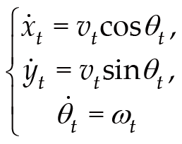
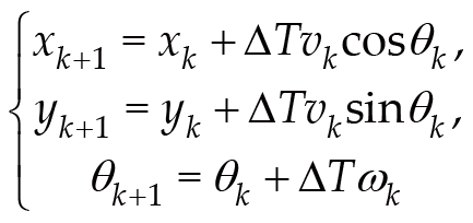
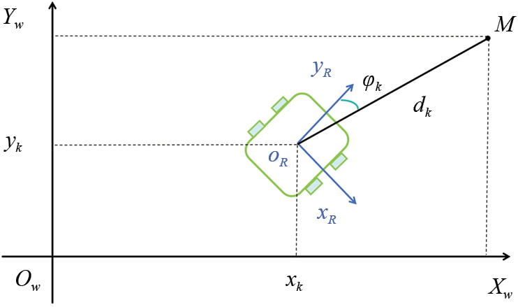
In this study, a mobile wheeled robot, as shown in Fig. 1, is considered. The kinematic model of the mobile robot can be described as follows:(1)where (xt, yt) represents the position of the mobile robot and θt denotes its orientation angle, which is defined as the angle between the robot's forward axis yR and xw axis. The displacement velocity vt and angular velocity ωt of the mobile robot can be obtained from odometric measurements. We assume that these velocities remain constant over the sampling period. Based on this assumption, the continuous-time system (1) can be discretized as follows:(2)where ΔT is the sampling period.
By defining and  , and taking into account external disturbances and random faults, the robot systems
can be reformulated as follows:(3)where ϕk is a zero-mean Gaussian noise with covariances Rk>0, and is a known matrix with appropriate dimensions.
, and taking into account external disturbances and random faults, the robot systems
can be reformulated as follows:(3)where ϕk is a zero-mean Gaussian noise with covariances Rk>0, and is a known matrix with appropriate dimensions.
The variable αk represents the stochastic nature of the fault, and follows the Bernoulli distribution
given by: (4)where is a known scalar.
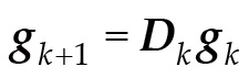
The dynamic characteristic of the fault gk is modeled as:(5)where Dk is a known matrix with appropriate dimensions.
Remark 1 This modeling choice is driven by the need to capture the stochastic nature of faults in real-world applications. As previously mentioned, faults in mobile robot localization systems stem from various uncertainties, including sensor degradation, environmental interference, and communication instability, making their occurrence inherently random. By representing fault dynamics with a linear stochastic process, we effectively model this randomness while maintaining mathematical simplicity and tractability. Moreover, this approach aligns with existing research in fault diagnosis and estimation, where similar stochastic models are widely adopted [10, 12].
Remark 2 The consideration of random faults in mobile robot localization arises from the complexity and uncertainty inherent in real-world environments. Sensors may experience random faults due to environmental interference or hardware degradation, while actuators are susceptible to anomalies caused by ground friction or sudden load changes. Traditional mobile robot localization methods often assume ideal conditions and overlook such faults. However, when these faults occur, they can lead to cumulative localization errors in mild cases, or even result in complete failure in severe cases. From an engineering perspective, accurately modeling and estimating these random faults can significantly enhance the reliability of mobile robot localization systems. Faults in a system refer to abnormal changes in its behavior or parameters that deviate from normal operation. These faults may result from hardware failures, sensor degradation, or external disturbances affecting system performance. In contrast, noise represents random interference or errors that distort measurements or disrupt system dynamics.
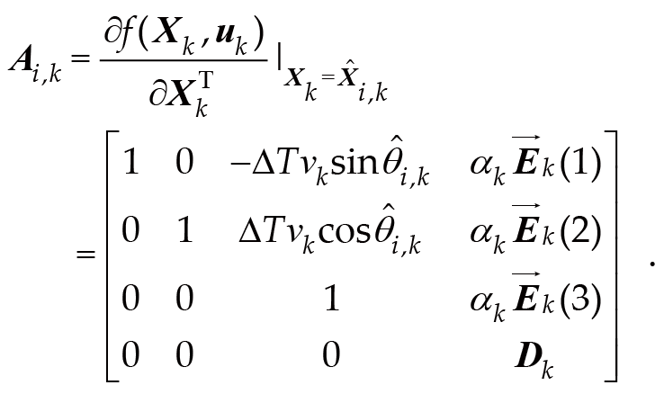
By defining and , the augmented system can be written as the following, derived from Eqs. (1) and
(5):(6)where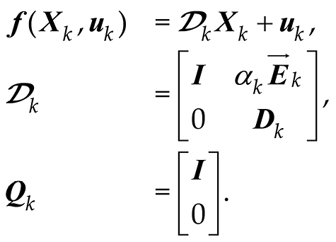
Before implementing the proposed mobile robot localization problem, it is necessary
to address the nonlinear system (Eq. (6)). Denoting the state estimation Xk as and expanding the nonlinear function around , Eq. (6) can be further expressed as: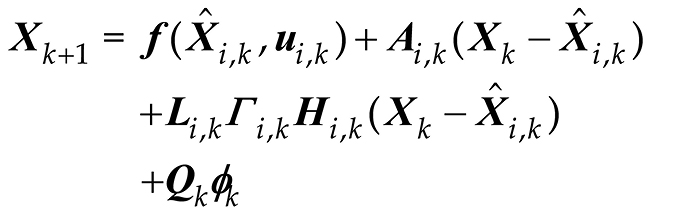 (7)whereLi,k is a scaling matrix associated with the system dynamics, while Hi,k is a matrix that provides an additional degree of freedom for estimator i. The uncertain matrix satisfies , which accounts for the linearization errors in the nonlinear system (6).
The initial value X0 is a Gaussian random variable with mean 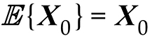 and covariance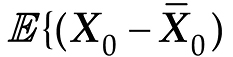
 , where is a given vector and R0 is a symmetric matrix.
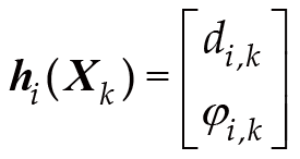
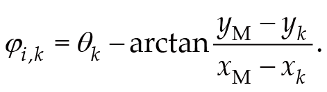
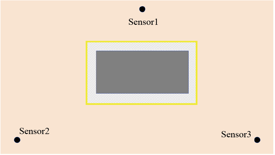
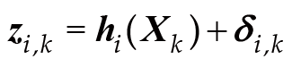
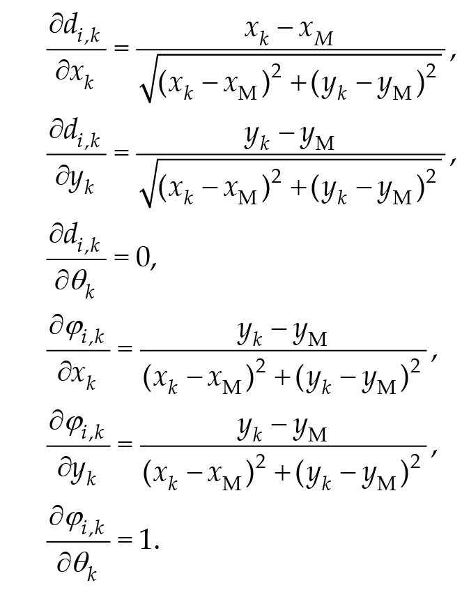
Sensor i, mounted on the mobile robot platform, consists of an energy harvester for collecting energy and a rechargeable device for storing and regulating the energy. The position of the sensors relative to the mobile robot is shown in Fig 2. At each time step k, the system's energy model is described by:(8)where the distance di,k between the robot's position (xk, yk) and a landmark M is given by:(9)where xM and yM denote the position of landmark M, and the azimuth φi,k is given by(10)
Taking measurement noise into account, the following measurement model is derived from Eq. (8):(11)where δi,k is a zero-mean Gaussian white-noise sequence with covariance Wi,k>0.
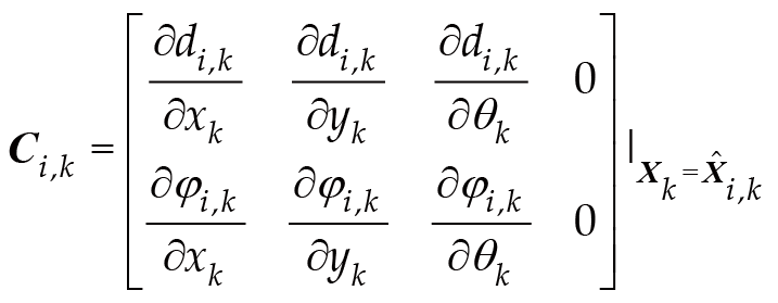
Applying the Taylor series expansion again, the nonlinear measurement model (Eq. (11))
can be described as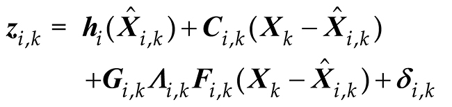 (12)wherewithGi,k is a scaling matrix associated with system dynamics, while Fi,k is a matrix that provide an additional degree of freedom for estimator i. The uncertain matrix satisfies , which accounts for the linearization errors in the nonlinear system (Eq. (11)).
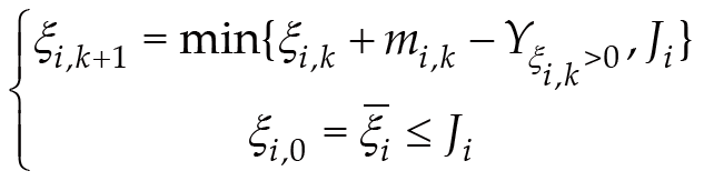
The energy collector i can obtain energy from the external environment, while the rechargeable device i stores the collected energy and powers the sensor i. At the time , the energy stored in the rechargeable device i is expressed as ξi,k∈{0,1,…,Ji}, where Ji represents the maximum amount of energy that the rechargeable device i can store. The energy mi,k collected by the energy collector at a time k is random and follows a probability distribution given by:(13)where and satisfies .
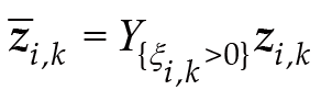
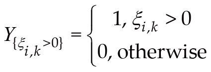
At time k, if ξi,k>0, the sensor i can send its measurement to the estimator i while consuming one energy measurement unit. Thus, the energy-level dynamics of the rechargeable device i can be described as:(14)and the measurement obtained by the estimator i is given by:(15)where is an indicator function such that:(16)
Remark 3 Compared with conventional sensors used in mobile robot localization, this study employs an advanced sensor with energy harvesting capability to enhance localization performance. The energy harvester continuously absorbs energy from the external environment, significantly extending the sensor's operational lifespan. Notably, the amount of energy harvested at time instant k is random, meaning that mi,k=0 is a possible scenario. Moreover, regardless of the amount of energy harvested, the sensor consumes one unit of energy whenever ξi,k. Consequently, the ξi,k=0 may arise at certain time instances, leading to potential measurement unavailability.
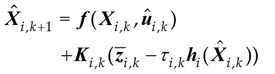
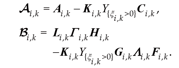
Assume that X0, ϕk, δi,k and mi,k are independent. To obtain local positioning information, a local estimator i of the following form is constructed:(17)where is the local estimate of estimator i, Ki,k is the estimator parameter of estimator i, and  .
.
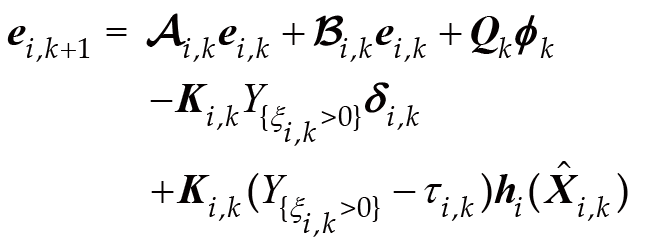
Let the localization error by , and we can derive the following error dynamic system:(18)where(19)We define the following localization error covariance matrix Pi,k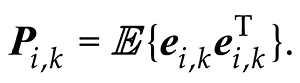 (20)
(20)
In this study, the main objective can be summarized as follows: (1) For each estimator i, we derive an upper bound Ξi,k such that Pi,k≤Ξi,k, and then determine the appropriate parameter Ki,k to minimize this upper bound; (2) The localization center utilizes the local position information from estimator i and applies an appropriate fusion estimation strategy to achieve mobile robot localization.
In this part, the mobile robot localization problem proposed is solved. Before proceeding further, the probability distribution σi,k for the energy level ξi,k of the rechargeable device i is calculated. Define σi,k as σi,k=[Pr{ξi,k=0} Pr{ξi,k=1}…Pr{ξi,k=Ji}]. The following Lemma will apply the recursive calculation method to find σi,k.
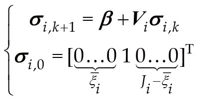
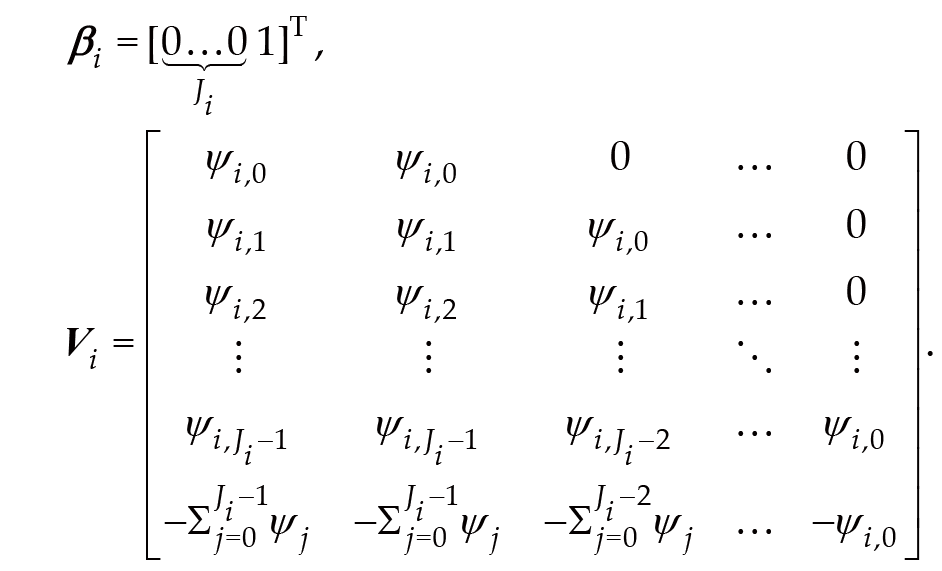
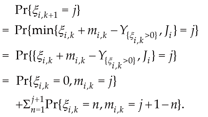
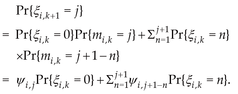
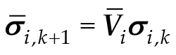
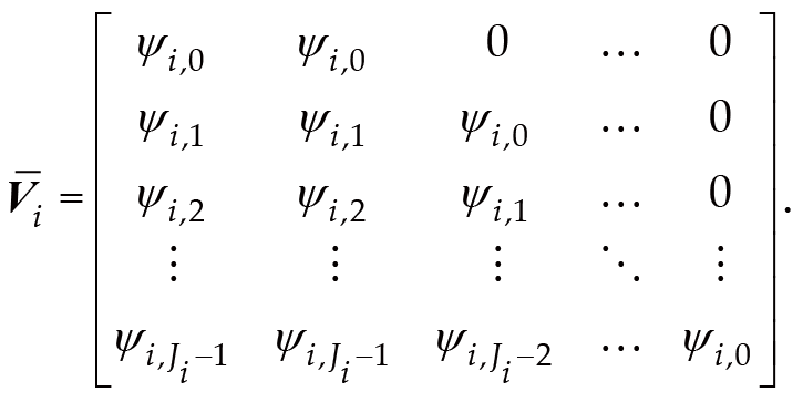
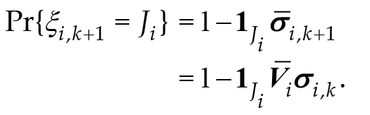
Lemma 1 According to the dynamic model of energy level ξi,k given in Eq. (14), the recursion of its probability distribution σi,k can be expressed as(21)whereProof. According to Eq. (14), the probability of ξi,k+1=j(0≤j<Ji) can be calculated as follows:(22)Note ξi,k and mi,k are independent of each other, and Eq. (22) can be further written as(23)Define . Obtained by Eq. (23):(24)whereThe probability of ξi,k+1=Ji can then be given by the following equation:(25)By combining Eqs. (24) and (25), the recursive Eq. (21) can be easily obtained. This Lemma proof ends.
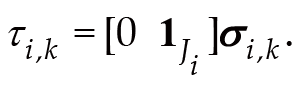
In the case of sensor i with energy harvesting function, according to Lemma 1, the expected value of the sensor's measured transmission can be calculated by:(26)
In the next Theorem, we obtain an upper bound Ξi,k for the matrix Pi,k and then minimized by appropriately choosing the estimator parameter.
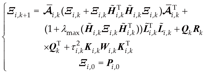
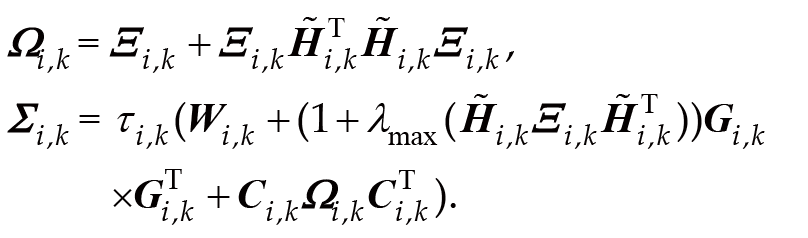
Theorem 1 Consider the system Eq. (6) and the local estimator Eq. (17). If the matrices Ξi,k satisfy the following recursion:(27)where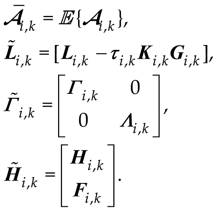 Then, the covariance matrix Pi,k is bounded by the matrix Ξi,k, that is, Pi,k≤Ξi,k.
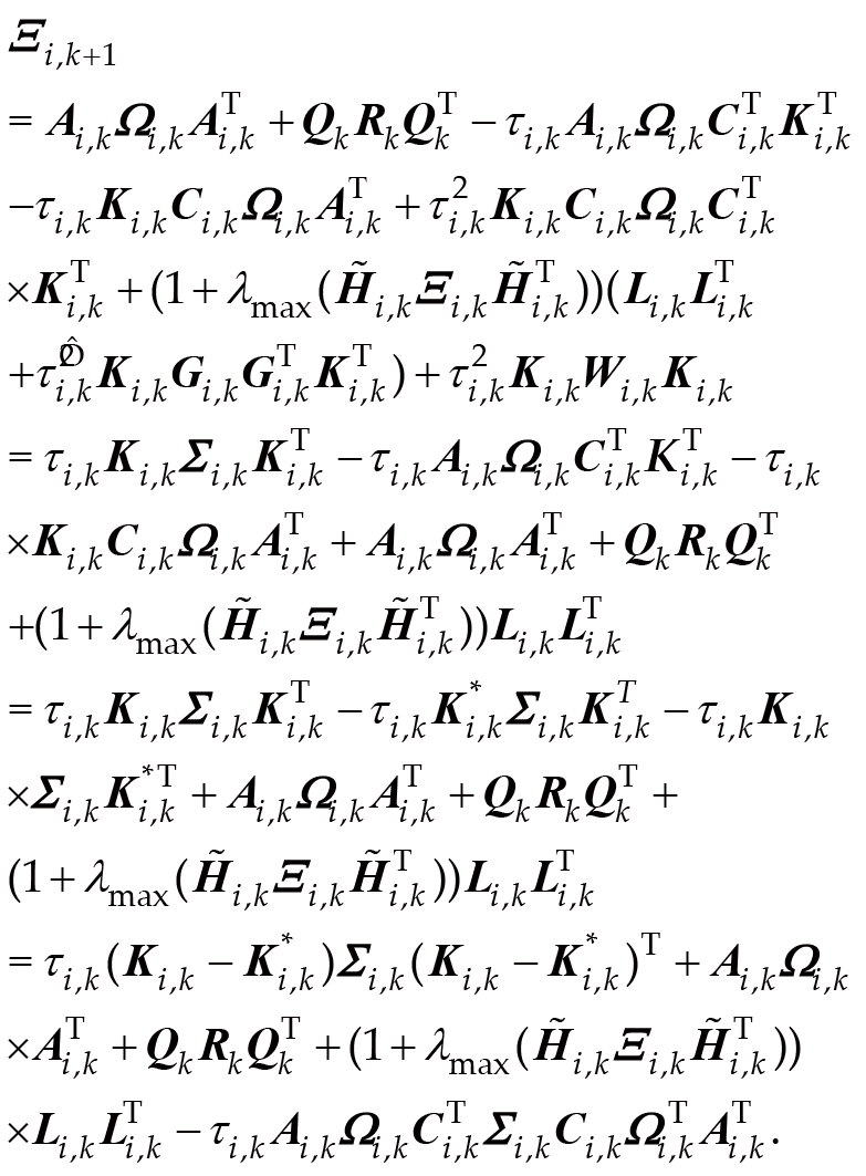
Furthermore, the local estimator parameter Ki,k can be designed to minimize the upper bound Ξi,k as follows:(28)whereProof. We use the mathematical induction to prove this Theorem. It can be obtained from
the initial condition that Pi,0≤Ξi,0. Assuming Pi,k≤Ξi,k, we need to show that Pi,k+1≤Ξi,k+1.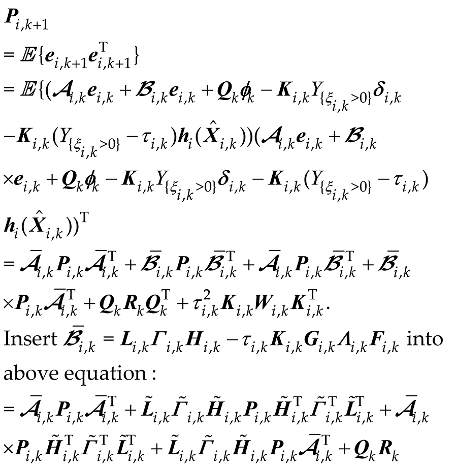
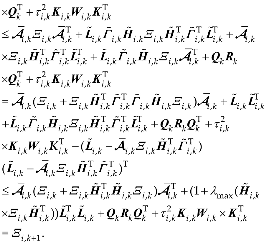 Insert
  into the above equation:(29)When , Ξi,k takes the minimum value, that is (Ξi,k)min(30)The proof is completed.
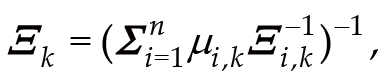
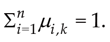
and Ξk are defined as the fusion positioning information and the fusion positioning error covariance, respectively. To achieve this purpose, the following fusion solution is adopted.(31)(32)where μi,k>0 satisfies(33)
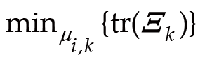
Consequently, the fusion estimation problem can be cast as a convex optimization framework with the following structure.(34)(35)
Theorem 2 Considering the argument system (Eq. (6)) and the local estimator (Eq. (17)), the
fusion estimation scheme adopted is consistent with Eqs. (34)–(38), i.e., (36)Proof. From Theorem 1, we have Pi,k≤Ξi,k. Combining the results in Eq. (26), and thus we can draw the conclusion that Eq.
(36) is valid. We omit the proof for brevity.
(36)Proof. From Theorem 1, we have Pi,k≤Ξi,k. Combining the results in Eq. (26), and thus we can draw the conclusion that Eq.
(36) is valid. We omit the proof for brevity.
Remark 4 Based on the preceding analysis, Theorem 1 derives an upper bound for Pi,k, and the estimator parameter Ki,k is obtained by minimizing this upper bound Ξi,k. Theorem 2 proposes a mobile robot localization scheme that employs a covariance intersection fusion estimation method, utilizing local positioning information and the minimized local upper bound Ξi,k. As a result, the joint state and fault fusion estimation problem for mobile robot localization with energy harvesting sensors is effectively addressed. The proposed algorithm for mobile robot localization is described as follows.
Algorithm: Mobile robot localization algorithm
(1) Set the parameters of the mobile robot system, initial values X0, Ξi,0, , the finite-horizon length N and k=0;
(2) Compute the fusion estimate and its covariance Ξk by Eqs. (34)–(35);
(3) Compute the estimator parameter Ki,k by (28), local estimate via (17), and local upper bound Ξi,k+1 according to Eq. (27);
(4) If k≤N, set k=k+1 and return to Step 2, else go to Step 5;
(5) Stop;
Remark 5 The practical applications of this paper can be summarized as follows: (1) Enhanced robustness in mobile robot localization: the proposed method integrates state estimation with fault-tolerant fusion, improving localization accuracy and stability even in the presence of intermittent sensor failures and energy-limited conditions. This is particularly beneficial for autonomous navigation, intelligent transportation, and drone control applications. (2) Adaptability to energy-constrained environments: the study introduces a novel localization approach designed for energy-harvesting sensors, ensuring reliable estimation even when sensor measurements are lost due to energy depletion. This is crucial for long-term autonomous systems, including deep-sea exploration robots, drone swarms, and space probes. (3) Innovative multi-sensor fusion: the use of the covariance intersection fusion method effectively integrates multiple local estimates, enhancing localization accuracy while reducing computational complexity. This approach is highly suitable for large-scale sensor networks and complex robotic systems, such as warehouse automation and agricultural robotics.
In this section, the effectiveness of the proposed mobile robot localization algorithm is demonstrated.
N=210 is denoted by the finite horizon. The sampling period of the mobile robot's odometer is 150 ms. The angular velocity is set by 0.2 rad/s, and the displacement velocity is 400 mm/s. The covariance matrices are defined as Rk=0.01I and Wi,k=0.01I(i=1,2,3), respectively. The other parameters in this scheme can be selected by: Li,k=[0.1 0.1 0.1 0.1]T (i=1,2,3), Hi,k=[0.1 0.1 0.1 0.1] (i=1,2,3), Gi,k=[0.01 0.01]T (i=1,2,3), Fi,k=[0.1 0.1 0.1 0.1] (i=1,2,3), and Dk=2sin(k). The random variable is chosen to be 0.95, and landmark position M is selected as M (xM=8 m, yM=8 m).
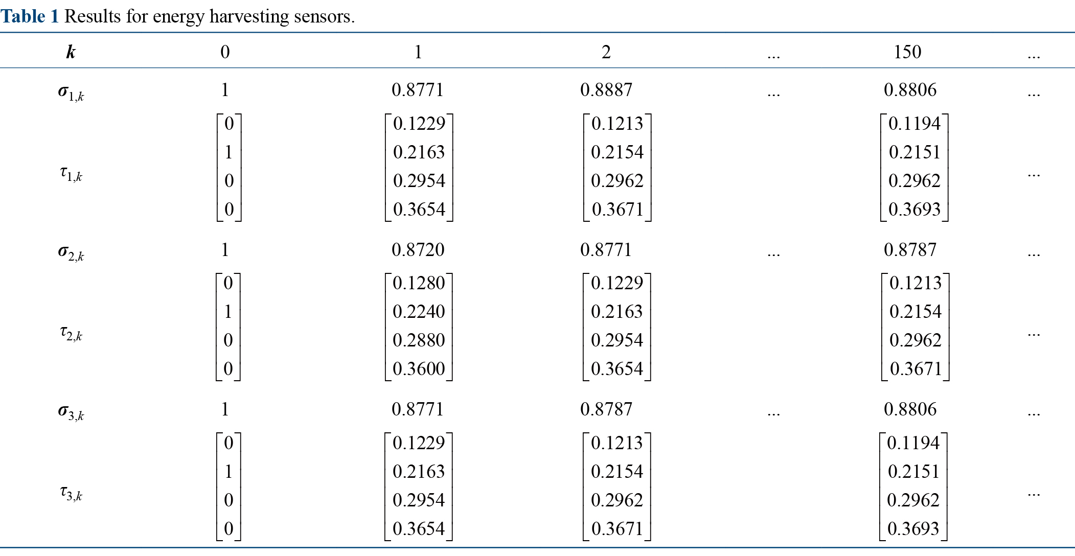
The sensor, equipped with an energy harvesting function, is assumed to be the maximum energy level Ji=3 that can be stored by the rechargeable device. The initial energy stored in the device is , where . At each instant, the energy collected by the energy harvester follows an independent and identically distributed Poisson distribution, i.e., Prob(mi,k=j)=, where λk=1. Based on the results from Lemma 1, the probability distribution σi,k and the expected value τi,k of the stored energy level of a rechargeable device can be calculated recursively. The recursive computation process for both the probability distribution σi,k(i=1,2,3) and the expected value of measurement transmission τi,k(i=1,2,3) is illustrated in Table 1.
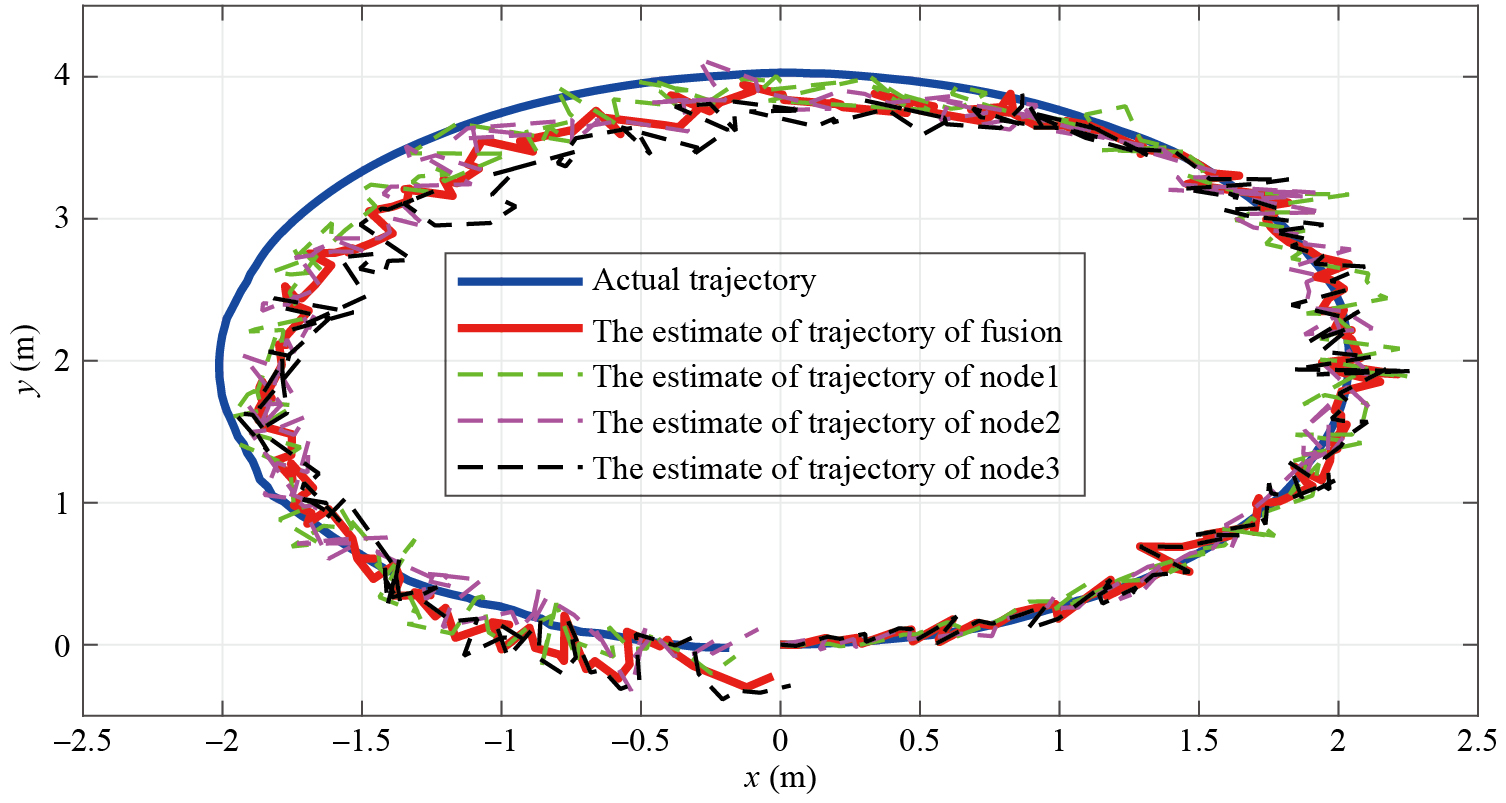
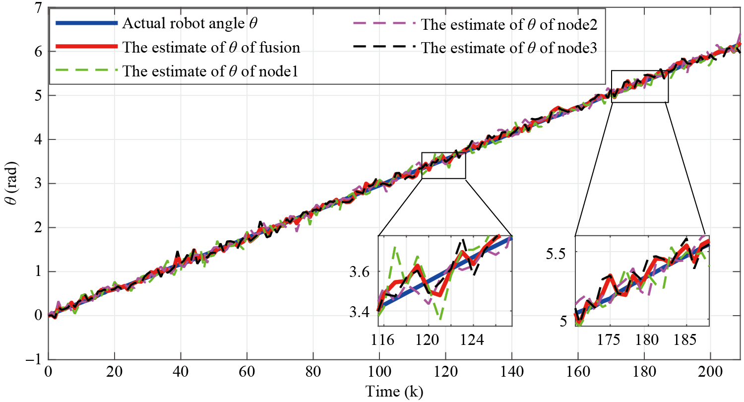
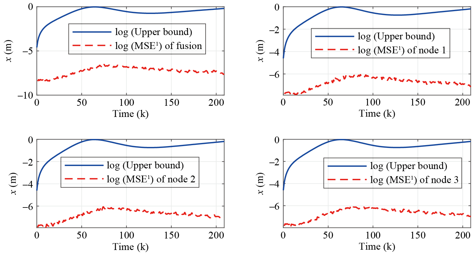
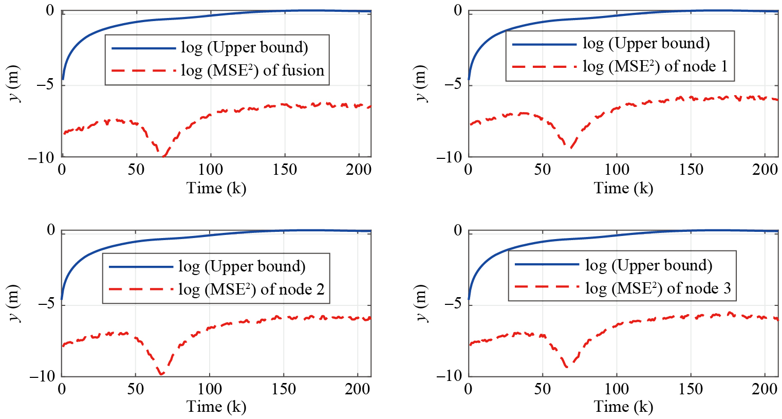
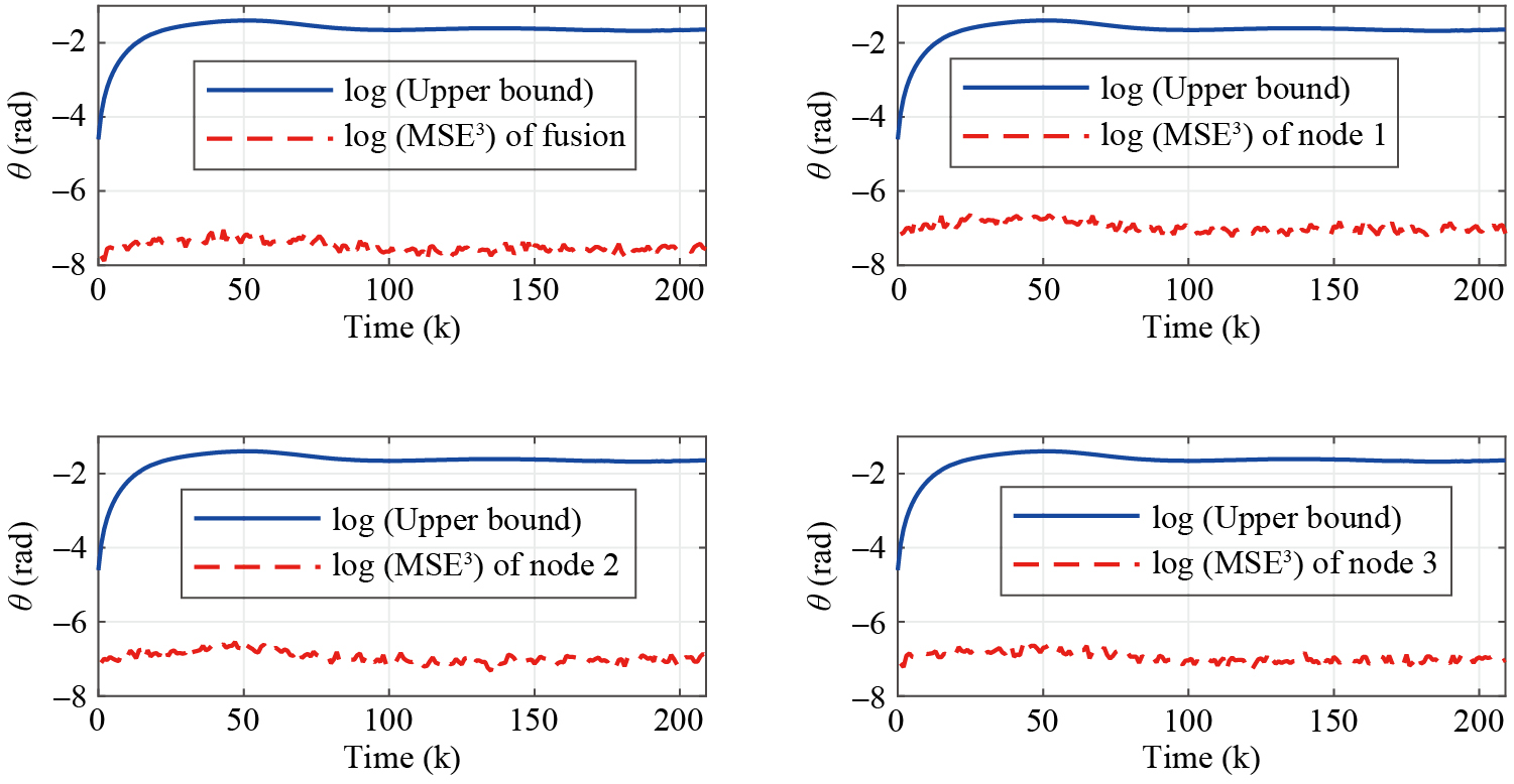
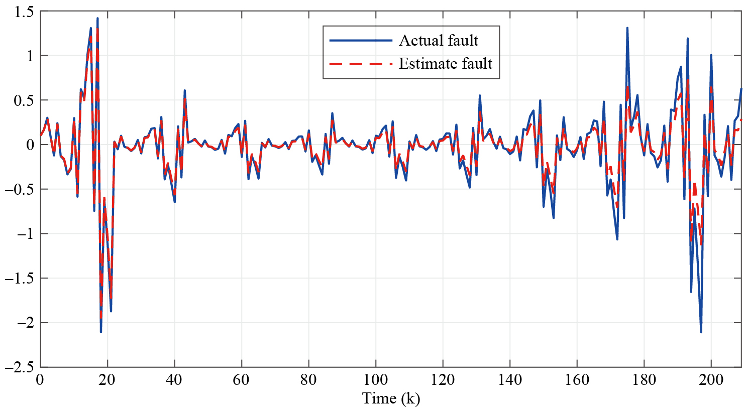
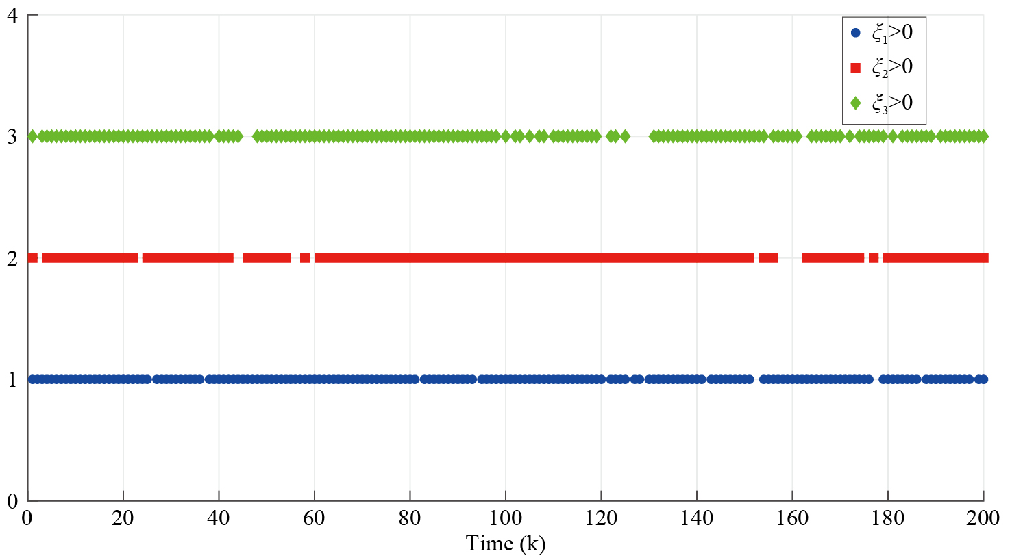
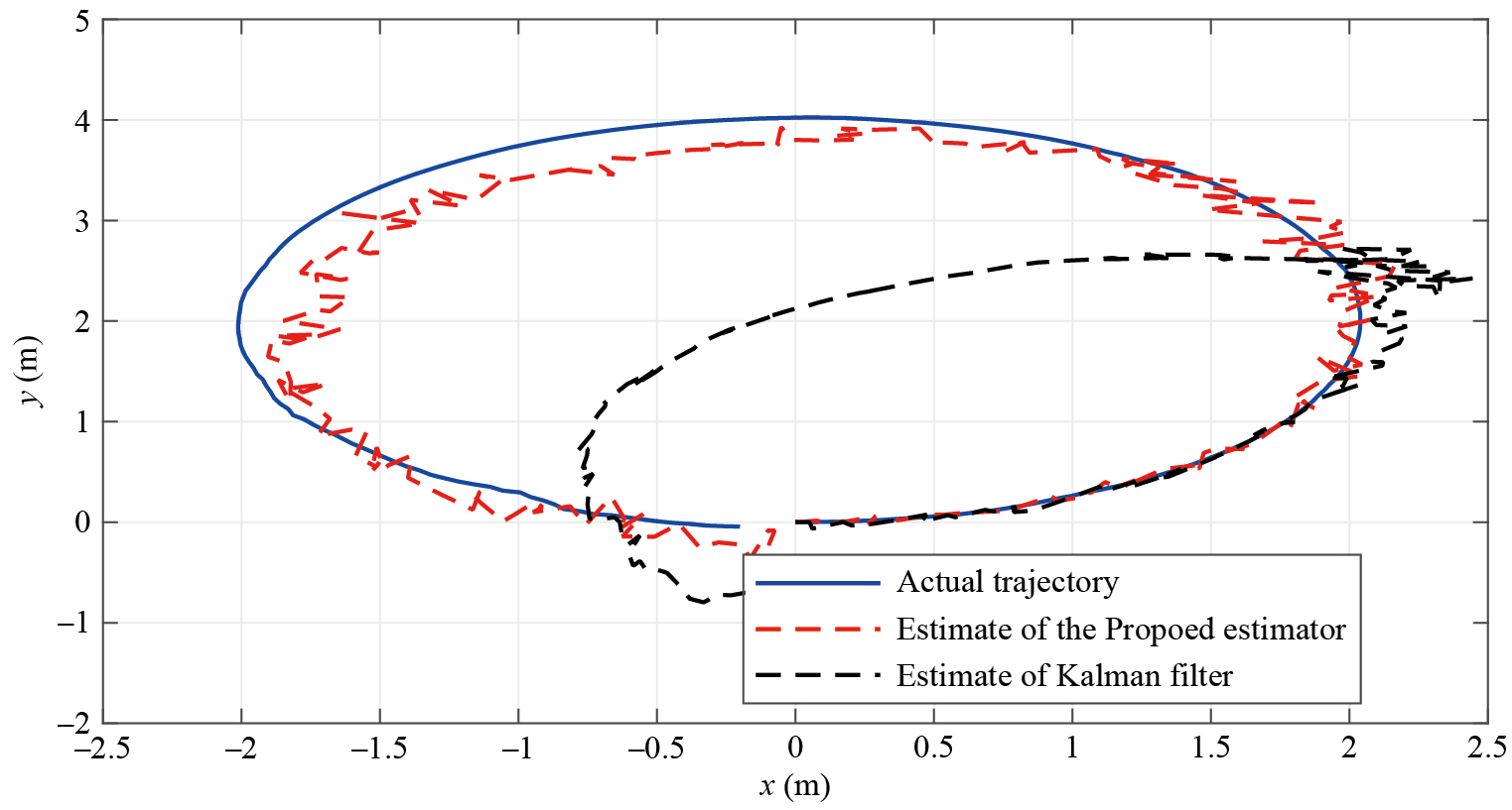
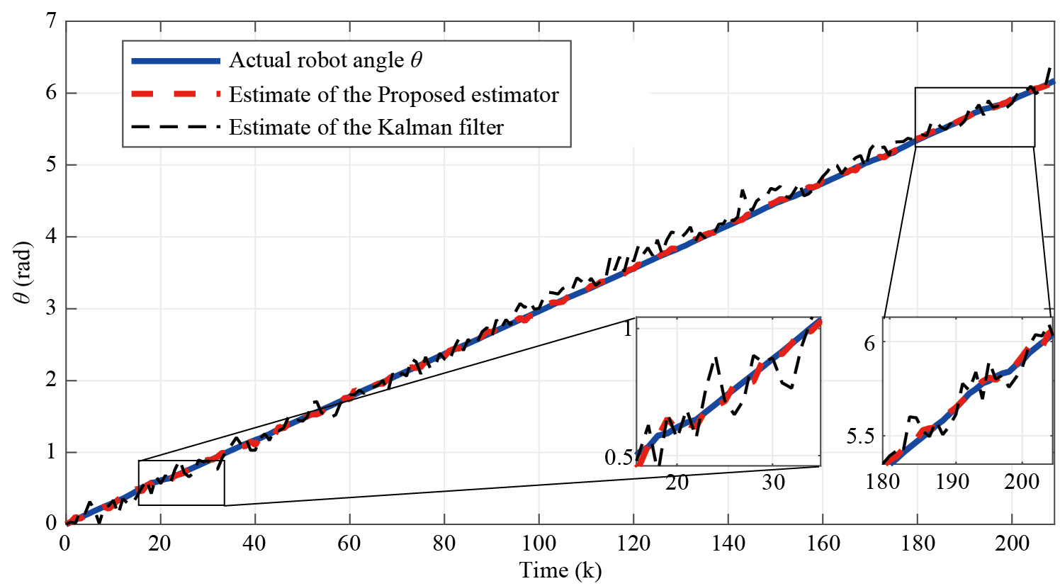
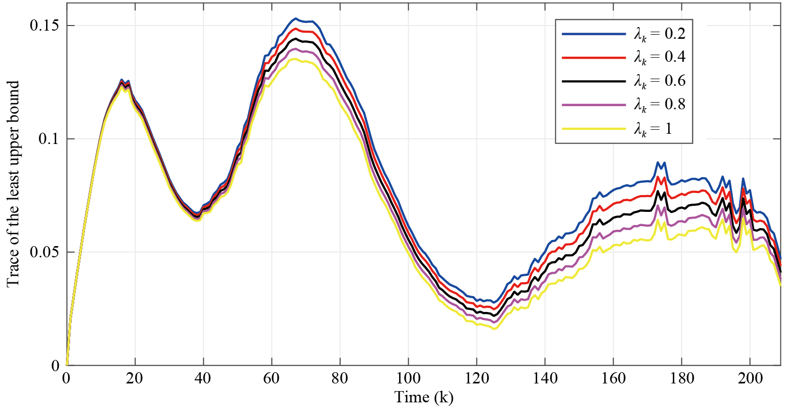
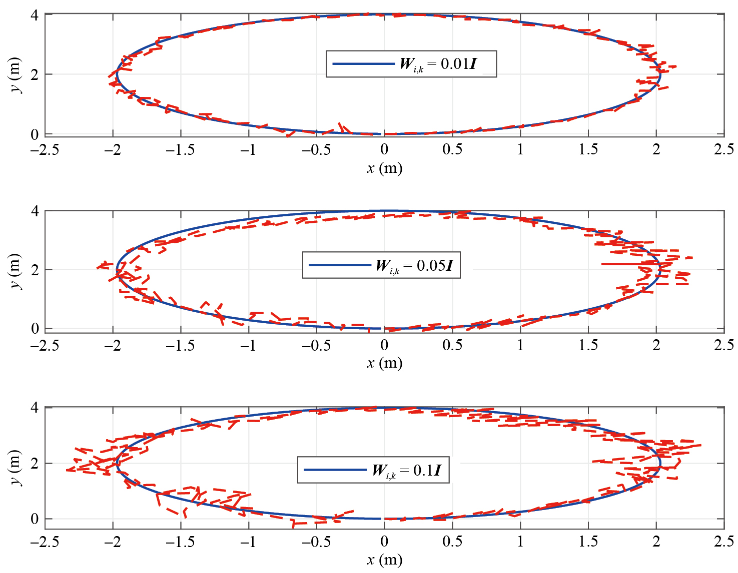
The main results are shown in Figs. 3–13. Figure 3 illustrates the actual trajectory of the robot and its estimates of local estimators. The 1st subplot in Fig. 5 draws the mean square error (MSE, defined by ) and their upper bounds of fusion estimation, the rest subplots in Fig. 5 plot the same thing in the 1st subplot. The fault signal and its corresponding estimate are shown in Fig. 8. Moreover, Fig. 9 illustrates the moments ξi,k>0. Figures 10–11 demonstrate that the proposed solution outperforms the conventional Kalman filter under the complex circumstances considered in this study. Finally, Fig. 12 reveals the impact of the parameter λk on the positioning performance, with a comparison of the minimum upper bound trace of different values of λk. As shown in Fig. 12, a larger λk results in a smaller trace of the upper bound Ξk, which aligns with the actual system behavior. To more effectively evaluate the robustness of the proposed algorithm, Fig. 13 presents its estimation performance under three distinct noise concentration levels: low, medium, and high.
Remark 6 The Poisson distribution is a discrete distribution that effectively captures the randomness and sparsity of energy arrivals. In energy harvesting scenarios such as solar or vibration-based systems, arrivals are often discontinuous, with some time intervals receiving no energy. The Poisson distribution naturally accommodates zero arrivals, making it well-suited for modeling real-world energy harvesting processes [13, 16]. In contrast, the uniform distribution assumes evenly distributed energy arrivals within a fixed range, which does not reflect real-world conditions. Energy arrivals in natural environments are typically sparse and irregular, making the uniform distribution inadequate [14]. Similarly, the Gaussian distribution is primarily used for continuous variables, whereas harvested energy is typically discrete. Additionally, the Gaussian model assumes a symmetric distribution around the mean, which fails to capture the inherent randomness and fluctuations of energy harvesting. Among these models, the Poisson distribution most accurately represents the stochastic and sparse nature of energy arrivals, particularly in low-energy scenarios [15, 20].
Based on the preceding simulation results and discussions, it is clear that the designed estimator performs well for the proposed mobile robot localization problem, demonstrating its effectiveness.
This study presents a joint state and fault fusion estimation scheme for mobile robot localization using energy harvesting sensors. A random variable following known probability distributions is employed to model fault randomness. The rate of measurement loss induced by sensor energy depletion is derived. In the presence of both energy-induced measurement loss and random faults, a local upper bound is guaranteed and minimized by optimizing the local estimator parameter. Furthermore, local estimates are fused using the covariance intersection method. Experimental results validate the effectiveness of the proposed estimation scheme. Future research may explore mobile robot localization under denial-of-service (DoS) attacks [21] and within dynamic event-triggered mechanisms [7].
This work was supported in part by the National Natural Science Foundation of China (Nos. 62403259, 62431014, and 62001254), the Natural Science Foundation of Jiangsu Province (No. BK20240945), Fujian Province Special Fund Project for Promoting High-Quality Development of Marine and Fisheries Industries (No. FJHYF-ZH-2023-03), and the Natural Science Foundation of Nantong (No. JC2023074).
G. Calafiore, "Reliable localization using set-valued nonlinear filters," IEEE Transactions on Systems, Man, and Cybernetics-Part A: Systems and Humans, vol. 35, no. 2, pp. 189–197, 2005.
R. P. Guan, B. Ristic, L. Wang, and R. Evans, "Monte Carlo localisation of a mobile robot using a doppler-azimuth radar," Automatica, vol. 97, pp. 161–166, 2018.
R. Havangi, "Mobile robot localization based on PSO estimator," Asian Journal of Control, vol. 21, no. 4, pp. 2167–2178, 2019.
Y. Lu and B. Shen, "Mobile robot localization under stochastic communication protocol," Kybernetika, vol. 56, no. 1, pp. 152–169, 2020.
Q. Sun, Y. Tian, and M. Diao, "Cooperative localization algorithm based on hybrid topology architecture for multiple mobile robot system," IEEE Internet of Things Journal, vol. 5, no. 6, pp. 4753–4763, 2018.
H. Dong, Z. Wang, S. Ding, and H. Gao, "Finite-horizon estimation of randomly occurring faults for a class of nonlinear time-varying systems," Automatica, vol. 50, no. 12, pp. 3182–3189, 2014.
C. Huang, S. Coskun, X. Zhang, and P. Mei, "State and fault estimation for nonlinear systems subject to censored measurements: A dynamic event-triggered case," International Journal of Robust Nonlinear Control, vol. 32, no. 8, pp. 4946–4965, 2022.
C. Huang, B. Shen, L, Zou, and Y. Shen, "Event-triggering state and fault estimation for a class of nonlinear systems subject to sensor saturations," Sensors, vol. 21, no. 4, p. 1242, 2021.
X. Bu, H. Dong, Z. Wang, and H. Liu, "Non-fragile distributed fault estimation for a class of nonlinear time-varying systems over sensor networks: The finite-horizon case," IEEE Transactions on Signal and Information Processing over Networks, vol. 5, no. 1, pp. 61–69, 2019.
C. Lo, J. P. Lynch, and M. Liu, "Distributed model-based nonlinear sensor fault diagnosis in wireless sensor networks," Mechanical Systems and Signal Processing, vol. 66. pp. 470–484, 2015.
Z. Gao, X. Liu, and M. Z. Q. Chen, "Unknown input observer-based robust fault estimation for systems corrupted by partially decoupled disturbances," IEEE Transactions on Industrial Electronics, vol. 63, no. 4, pp. 2537–2547, 2016.
J. Yan, C. Deng, W. Che, and X. Liu, "Fault estimation for cyber-physical systems with intermittent measurement transmissions via a hybrid observer approach," Journal of the Franklin Institute, vol. 361, no. 3, pp. 1497–1509, 2024.
Y. Li, F. Zhang, D. Quevedo, V. Lau, S. Dey, and L. Shi, "Power control of an energy harvesting sensor of remote state estimation," IEEE Transactions on Automatic Control, vol. 62, no. 1, pp. 277–290, 2016.
C. Ho and R. Zhang, "Optimal energy allocation for wireless communications with energy harvesting constraints," IEEE Transactions on Signal Processing, vol. 60, no. 9, pp. 4808–4818, 2012.
E. Bitar, R. Rajagopal, P. Khargonekar, K. Poolla, and P. varaiya, "Bringing wind energy to market," IEEE Transactions on Power Systems, vol. 27, no. 3, pp. 1225–1235, 2012.
A. Hentati, J. Frigon, and W. Ajib, "Energy harvesting wireless sensor networks with channel estimation: Delay and packet loss performance analysis," IEEE Transactions on Vehicular Technology, vol. 69, no. 2, pp. 1956–1969, 2020.
M. Calvo-Fullana, C. Anton-Haro, J. Mathmoros, and A. Ribeiro, "Random access communication for wireless control systems with energy harvesting sensors," IEEE Transactions on Signal Processing, vol. 68, pp. 3961–3975, 2020.
X. Bao, H. Liang, Y. Liu, and F. Zhang, "A stochastic game approach for collaborative beam-forming in SDN-based energy harvesting wireless sensor networks," IEEE Internet of Things Journal, vol. 6, no. 6, pp. 9583–9595, 2019.
B. Shen, Z. Wang, D. Wang, J. Luo, H. Pu, and Y. Peng, "Finite-horizon filtering for a class of nonlinear time-delayed systems with an energy harvesting sensor," Automatica, vol. 100, pp. 144–152, 2019.
J. Huang, D. Shi, and T. Chen, "Event-triggered state estimation with an energy harvesting sensor," IEEE Transactions on Automatic Control, vol. 62, no. 9, pp. 4768–4775, 2017.
D. Ye and Y. Sang, "Optimal periodic DoS attack with energy harvester in cyber-physical systems," Neurocomputing, vol. 390, pp. 69–77, 2020.
W. Song, Z. Wang, J. Wang, F. E. Alsaadi, and J. Shan, "Particle filtering for nonlinear/non-Gaussian systems with energy harvesting sensors subject to randomly occuring sensor saturations," IEEE Transactions on Signal Processing, vol. 69, pp. 15–27, 2020.
A. Canedo-Rodriguez, V. Alvares-Santos, C. V. Reguerio, R. Iglesias, S. Barro, and J. Presedo, "Practicle filter robot localization through robust fusion of laser, WiFi, compass, and a network of external carneras," Information Fusion, vol. 27, pp. 170–188, 2016.
L. Jetto, S. Longhi, and D. Vitali, "Localization of a wheeled mobile robot by sensor data fusion based on fuzzy logic adapted Kalman filter," Control Engineering Practice, vol. 7, no. 6, pp. 763–771, 1999.
H. Zhu and M. Luo, "Hybrid robust sequential fusion estimation for WSN-assisted moving-target localization with sensor-node-position uncertainty," IEEE Transactions on Instrumentation and Measurement, vol. 69, no. 9, pp. 6499–6508, 2020.
Z. Deng, P. Zhang, W. Qi, Y. Gao, and J. Liu, "The accuracy comparison of multisensor covariance intersection fuser and three weighting fusers," Information Fusion, vol. 14, no. 2, pp. 177–185, 2013.
H. Geng, Y. Liang, and X. Zhang, "Linear-minimum-mean-square-error observer for multi-rate sensor fusion with missing measurements," IET Control Theory & Applications, vol. 8, no. 14, pp. 1375–1383, 2014.
C. Ran and Z. Deng, "Robust fusion Kalman estimators for networked mixed uncertain systems with random one-step measurement delays, missing measurements, multiplicative noises and uncertain noise variances," Information Sciences, vol. 534, pp. 27–52, 2020.
X. Feng, C. Wen, and J. H. Park, "Sequential fusion filtering for multi-rate multi-sensor time-varying systems-A Krein-space approach," IET Control Theory & Applications, vol. 11, no. 3, pp. 369–381, 2017.
 Top
Top