ContentsFigures & Tables
The development of intelligent driving technology has increased the safety challenge of vehicle system functions in the face of risky driving environments. Since the evaluation method based on mileage cannot meet the requirements of increasingly complex functional development and verification, the driving scene theory has gradually been recognized and studied worldwide. The driving scenario concept originated from the German PEGASUS project [1], and the simulation and verification standards for autonomous driving scenarios such as United Nations WP29, ISO Working Group on Autonomous Driving Test Scenarios, and ASAM OpenX series have also made continuous contributions to its development [2, 3].
Currently, there are numerous studies on the generation of test scenarios, which not only include methods based on artificial potential field (APF) but also encompass other advanced scenario generation methods such as those based on Bayesian networks, reinforcement learning, and deep learning. These methods each demonstrate unique strengths and limitations in the simulation and testing of intelligent driving systems. To comprehensively present the latest advancements in this field, it is essential to introduce and summarize these diverse approaches. However, the above driving scenarios are generally based on the subdivision of the traffic participating environment (road information, permanent and temporary traffic facilities, target objects, natural and artificial environments, digital basic information, etc.) and the behavior of the traffic participating objects, so as to build a simulation environment and carry out a large number of pass verification for a single function of the test system. It does not deeply involve the direct or indirect interaction between various traffic participants, traffic rules, drivers' subjective strategies, driving conditions and other factors in the real complex traffic environment, and the resultant comprehensive influence on driving participants. Therefore, the existing scenario construction and evaluation system is not enough to make a normalized analysis of the comprehensive effect of the intelligent driving system in its operational range, especially the impact of individual dangerous scenarios.
Higher-level intelligent driving systems (L3 and above) should deal with dynamic and complex interaction scene information in real time, consider not only the independent actions of traffic participants, but also the interaction between groups and the restriction of abstract rules, and make strategic support for their own intelligent driving vehicles based on accurate perception and accurate prediction. It is a prerequisite to ensure reasonable and safe driving in complex and changing scenes with random dynamic evolution. Due to the uncertainty of the environment and the driver's intention, the vehicle trajectory presents multi-modal attributes, that is, under the condition of the same historical trajectory, the future trajectory of the vehicle has multiple possibilities. Under the premise of considering the change of the scene, using the action field theory, the research of vehicle multimodal trajectory is one of the key fields of intelligent driving.
In order to more comprehensively describe the influence of group interaction on vehicle behavior, the method of APF came into being. Khatib regarded the motion space of autonomous vehicles as the potential field of superposition of the gravitational field from the destination and the repulsive field from the obstacle [4]. The gravitational force points to the destination and increases with the distance between the vehicle and the destination. In the motion space, the repulsion force generated by the obstacle is opposite to the direction of the obstacle and decreases as the distance between the obstacle and the vehicle increases [5]. The artificial potential field method has the advantages of fast planning speed and good obstacle avoidance effect, but it ignores the motion of dynamic obstacles and has problems such as trajectory oscillation [6, 7]. Therefore, some scholars have introduced more complex field theories to explain the distribution of attraction and repulsion forces in the whole area under the motion of obstacles.
In the 1920s, the formal concept of field theory was born, which pointed out that it is not the charges or particles of matter that are crucial for the description of physical phenomena, but the fields in the space in which they reside [8]. Einstein [10] proposed that space is a distribution system of forces, which determines what actions will be produced by objects with certain properties [9]. When applied to social domains involving complex cooperation and competition, the understanding of individual behavior requires an understanding of the context in which the behavior takes place (the status quo) and the various factors that affect the individual at a given time, that is, the totality and complexity of the presence. Ji and Peng et al. constructed a virtual three-dimensional potential energy field to evaluate the dangerous driving state of vehicles [11]. Reng and Zheng et al. introduced virtual force field and proposed a path planning method for obstacle avoidance based on model prediction theory [12]. Xiu Caijing et al. used field theory to abstract vehicle navigation, and the comprehensive field composed of virtual space electric field and relative velocity reflected vehicle motion [13]. The above traffic field studies are mainly based on the direct risks caused by the target obstacles in the longitudinal and lateral directions of intelligent driving vehicles at a static time, which cannot reflect the changing trend of the field energy. Lewin believes that the field is constantly changing and adapting, and change and invariability should be the relative concepts of group activities occurring in different quantities at any given time. He defines the field as "the whole of interdependent coexistence facts", and the time and mode of changing group behaviors are "quasi-stationary equilibrium", which should tend to change continuously and affect the results of group behaviors [13, 14]. Therefore, it is necessary to propose a method that can comprehensively evaluate the continuous influence of the interaction field in the observable space on the behavior of the host vehicle.
The main contributions of this paper are summarized as follows:
(1) This study introduces the Kalman particle filtering theory for deriving high-dimensional traffic scenarios, addressing the limitations of current methods that heavily rely on subjective analysis and experiential settings.
(2) By analyzing the distribution of comprehensive energy fields in normalized scenes with various elements from different dimensions, the study defines benchmark scenes based on field energy theory.
(3) The study conducts multi-level research on processing high-dimensional spatial element data, including scene element processing level and target/self-vehicle signal level.
The rest of this paper is organized as: In Section 2, the basic definitions and corollaries of pan-scene and particle theory are introduced. Section 3 is the research of pan-scene energy field algorithm, including pan-scene energy extraction and transformation, target observation and tracking. Section 4 shows the simulation results and analysis. Section 5 presents the conclusion and future work of this paper.
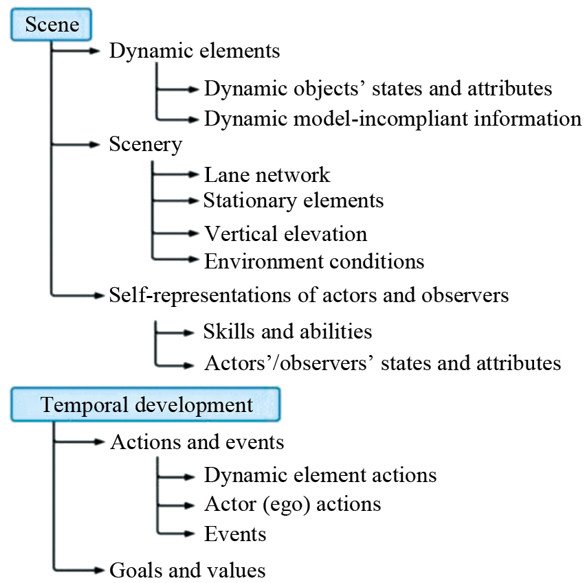
According to ISO 21448, a scenario is a description of the development in time domain between several scenarios in a series of scenes. A scenario is a snapshot of the environment, including scenery, dynamic elements, self-representation of all participants and observers, and the relationship between these entities [15], as shown in Fig. 1.
In the pan-scene system, site boundary conditions are the basic characteristics of the entire behavioral activity space. The range of the boundary depends on the individual observation, including the perception of the observation system and the personality, motivation and cognitive structure of the natural person. Therefore, the field is also the "activity space" of individuals [16]. The activity space is not the same as the geographical environment, the activity space is subjective, that is, it must be perceived by the participating individuals.
Therefore, based on the above theory, the pan-scenario system defines the scenario, situation and scenario expansion as follows:
A "scenario" describes a "slice" of the surrounding environment. The "scene" describes the static elements that constitute the situation, while the abstract description such as the dynamic trend of elements, the states of participants and observers, and the relations between all these entity elements can be summarized by the "emotion". Only in the simulation environment, all the situation information (including objective situation information and its true value) can be expressed objectively and accurately. However, in the real world, the situation information obtained from one or several observation angles (subjective situation) is doomed to be incomplete, incorrect and uncertain.
Among them, the static meta information and all other abstract information are combined into the real world slice to form the collection of all information.
For example, for a moment slice of a car-following scenario. Include possible static elements of host and target vehicles, lane lines, roads, dividers, and trees within the restricted orientation; However, the acceleration of the host vehicle, the activation of the auxiliary driving function, the braking behavior of the target vehicle, and the road reflection intensity can be regarded as other supplementary information.
The "situation" is the whole environment that needs to be considered to select an appropriate behavior pattern at a specific point in time, which includes all the conditions, observations, choices and executions related to the behavior. Situation is based on transient or permanent behavior goals and the vehicle's own driving ability, which is the screening and supplement of situation information. Thus, the "situation" from the perspective of an element is always "subjective".
A scenario describes the temporal development between several scenarios in a series of scenarios. Each scenario starts with an initial scenario. Actions and events and goals and evaluations can describe this temporal development in the scenario. Unlike a "scenario", a scenario must contain a certain time span.
The relationship between scenario, situation and scenario is as follows: The scenario can be seen as all the information collected through the original data; A situation is a relevant scenario for the behavior of an observer (e.g., a driving vehicle) extracted from a situation. A scenario is composed of a series of scenarios, and the elements contained in the scenario are filtered and combined for specific action and event analysis to meet the established goals and evaluation (such as functional verification of vehicles).
The concept of field can be intuitively described as the distribution of a physical quantity in a region of space. The field quantities at different points in space can be regarded as independent dynamic variables, and the field is a system with continuous infinite dimensional degrees of freedom. Field theory is the theory of the properties, interactions, and laws of motion of fields. A wave is an observable phenomenon caused by the propagation of a field. Microscopically, all matter can be seen as waves. At the macro level, a wave is a form of motion.
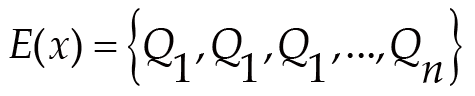
Extended to the driving ubiquitous scene theory, each element in the scene can constitute a virtual spatial field (such as speed field, etc.), then the information of a certain point in the spatial field can be described by calculating the energy intensity (speed) of each point in the space of the field, as shown in the formula:(1)where E(x) is the superposition energy space set and n is the number of elements Q included in this scene.
Energy is the sum of all kinds of energy in the pan-scene system, and its energy increases linearly with the activity of the system, and the larger the potential energy carries more transformable potential.
Pan-scene particle field theory is defined as follows.
(1) Each kind of event corresponds to a kind offield, and each field is ubiquitous in a specific scenario;
(2) when the field energy increases, the event (particle excitation) will be generated, and when the field energy decreases, the eventwill disappear (particle annihilation);
(3) there is no element of interest in the observed scene, which is the lowest pan-scene energy state, but there will still be random fluctuations;
(4) the definition of field does not depend on the lowest energy, while the definition of event depends on the lowest field energy;
(5) the field and its constituent elements (particles) have mass, energy, momentum and angular momentum changes as do the excitation events.
So the "gravitational field" comes from the energy excitation of the host vehicle by the destination; The traffic rule field comes from the energy excitation of the host vehicle movement behavior constraint by traffic rules. The hazard field comes from the excitation of energy to avoid the risk of collision and to reduce the expected collision hazard... The events of the pan-scene model are essentially derived from the energy excitation of various fields, and the pan-scene is the superposition of various field effects. Energy field and event are different observation angles in the same pan-scene. Field observes elements and their interactions from the perspective of space and energy, and event observes elements and their motion or transformation from the perspective of time and motion. The interaction of fields and fields drives the movement of objects and the change of events in this scene.
In the pan-scene data system, the basic scene data is transformed into the intelligent driving pan-scene particle energy field, and the Kalman particle filter method is used to extract the background and foreground of the pan-scene energy field. Through the verification of natural driving data, the comprehensive energy of the pan-scene system and the energy change caused by superposition events are described and verified.
ViBe algorithm is used to extract the data of each basic scene in the traffic pan-scene, and the energy distribution of particles in the traffic pan-scene is obtained. The steps are as follows:
(1) The superposition energy field E(x) at the initial time t0 is defined as Eq. (1);
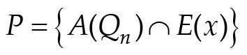
(2) compare and extract the energy changes of the above elements to the host vehicle at time t1(2)where P is the projection distance of each element Q in the initial energy space; A(Qx) is the circle centered at the centroid of the element Q and Rx is the radius.
In order to reduce the energy consumption of complex calculations, a phased collision avoidance region is established using the equipotential surface principle and fuzzy classification method.
(1) A0 is the expected collision area from the target element (traffic participating object), whose value is determined by the braking performance and the current relative speed. When the host vehicle touches and enters the area, it means that a collision occurs.
(2) A1 is the minimum safe area to avoid collision with the target element (traffic participating object). If the host vehicle is in this area, it means that the host vehicle is in an emergency state, which needs to be warned by the system and ready to make priority obstacle avoidance decisions to reduce the risk of collision.
(3) A2 is a safe area relatively far away from the target element (traffic participating object), and the host vehicle is currently free of collision risk. The main purpose is to drive to the destination while avoiding the risk of new collisions. It can be seen that there is a time interval t2 within which a direct jump from state A2 to state A1 or A0 is not possible.
(4) A3 is the "absolute" safe area away from the target element (the traffic participating object). There is a time interval t3 in which a direct jump from state A3 to state A2 cannot be made.
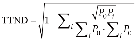
Here, the concept of virtual time-to-near-distance (TTND) between the observation object and other targets is introduced [17], and the element motion state (horizontal and vertical velocity, acceleration, steering, etc.) of the pan-scene event slice at the observation time is "frozen", and the motion vector of the main vehicle at the frozen time is kept unchanged [18–20]. Then it developed into the virtual trajectory collision with the target object, and used the hierarchical level of TTND to describe the energy field division distance between the main observation source object and other traffic participating objects, and adjusted the threshold division of the phased collision avoidance area according to the index [21].
The TTND calculation method is expressed in the formula:(3)where P0 is the corresponding initial energy value in the pan-scene energy field; Pi is the dynamic change value of energy in the dynamic development process of the scene.
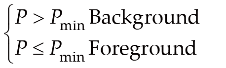
In the pan-scene energy field, due to the noise generated in the transformation process of the scene basic data, it is necessary to distinguish and extract the background and foreground in the energy field in order to pay more attention to the observed object in the energy field.
According to the energy extraction and comparison of the change of the host vehicle in Formula (2), the decision rule of setting a given threshold P min to judge the background and foreground of the pan-scene energy field is as follows [18].(4)
At the same time, it is necessary to randomly select a sample in the foreground model to replace the pixel value of the energy field to complete the real-time update and extraction of the foreground model.
Based on the above two stages of processing, the pan-scene energy field which is easy to observe is obtained. In order to meet the tracking and observation requirements of the target object in the pan-scene energy field, the Kalman particle filter method is used to construct the target state estimation and tracking model.
In order to better observe the observation object in the pan-scene energy field, it is assumed that the mathematical expression of the observation object state in the pan-scene energy field is as follows.(5)where xk represents the energy state of the observed object at the current time; A and B are the energy transfer matrix and energy control matrix, respectively. xk−1 represents the energy state of the observed object at the last time; uk−1 denote the energy Gaussian noise at the previous time. εk−1 denote the random environmental noise at the previous time instant.
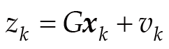
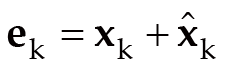
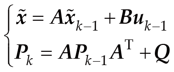
By constructing the observation model, the energy observation quantity can be obtained as follows.(6)where zk represents the observed energy quantity of the observed object; G represents the pan-scene energy field observation matrix. vk denote the energy observation noise. When the number of energy calculation iterations is k, the energy state estimation error of the observed object is as follows.(7)where ek represents the energy state estimation error of the observed object; denote the error correction value of the energy state estimation of the observed object. When the error of the observed state of the energy field is minimum, the state prediction equations of the observed object can be obtained, which is expressed as follows.(8)where represents the observation results after k−1 iterations; Pk represents the prediction result based on the energy state of the observed object; Q is the covariance of random environmental state noise, which is used to describe the value distribution law.
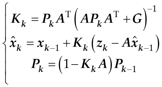
Similarly, the modified equation set of the energy state of the observed object in the pan-scene energy field is expressed as follows.(9)where Kk represents the correction control coefficient of pan-scene energy field; Pk denotes the corrected observed energy value of the observed object; is the revised energy estimate.
The constructed pan-scene energy field object observation model can accurately determine the energy state of the observed object, which provides support for the subsequent energy tracking of the observed object.
Through the observation of the energy state of the observed object in the pan-scene energy field in Section 3.3.1, the energy state of the observed object in the pan-scene can be tracked according to the principle of Kalman filter [22, 23]. The implementation steps are as follows:
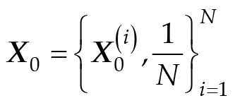
Select the observation object model, calculate its corresponding energy distribution, and construct the initial state particle sample set according to the energy distribution, which is expressed as:(10)
(1) Calculate the particle energy state transition, involving a new particle energy set as ;
(2) Calculate the particle distribution weight, and update the particle energy estimation results to xk;
(3) The uniformly distributed random number is used to update the particle energy set, and then a new particle energy set is generated.
(4) Repeat steps (2)–(4) above until the number of iterations is completed.
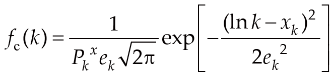
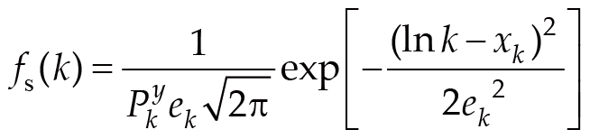
In the complex scene considering the interaction of traffic participants, the traffic strategy of repulsion caused by chain risk events and the comprehensive interaction field of the traffic destination are consistent with the real driving behavior, and the calculation method of the matching index of the predicted steering and longitudinal speed is as follows:(11)(12)where fc(k) and fs(k) are the predicted steering/lane change matching index and longitudinal speed matching index respectively; Pkx and Pky are the transverse and longitudinal components of the energy state of the observed object, respectively.
In summary, the Kalman particle filter method realizes the target observation and tracking in the pan-scene energy field, which provides sufficient preconditions for the research of driving behavior in the pan-scene energy field.
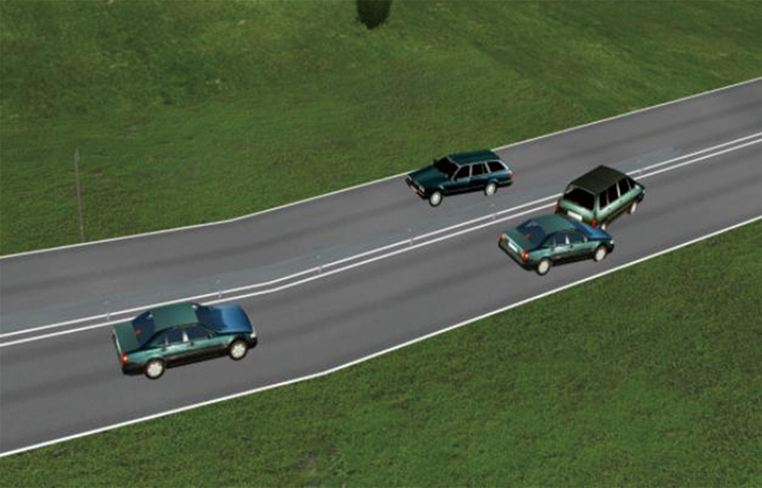
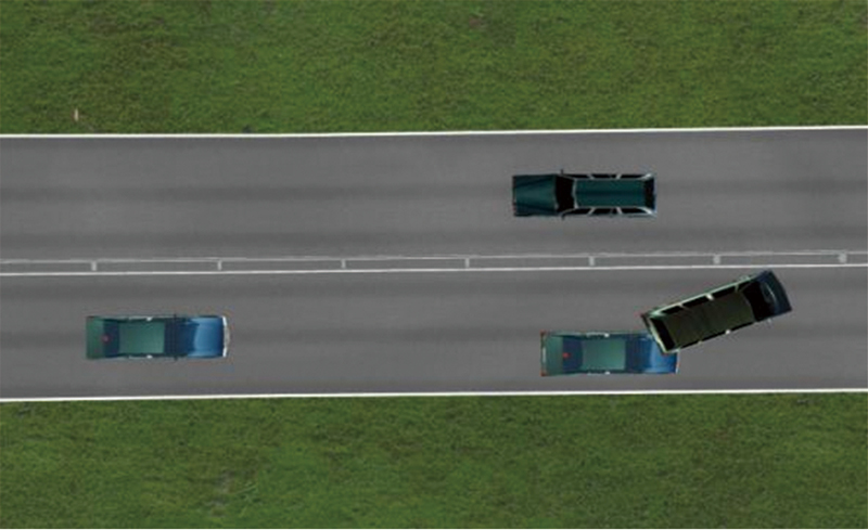
Based on the pan-scene energy field research algorithm proposed in this paper, this chapter carried out scene modeling through the scene simulation software VTD, as shown in Fig. 2 below. The traffic scene is a two-way single lane, the lane width is 5 m, and the road shape is depicted as a flat road plus a slope road (the slope is set to 10°). At the same time, there is a traffic accident in the right lane, and there is a car in the opposite direction in the left lane. The speed warning sign is set in the driving direction, and the driving speed is limited within 80 km/h. The road boundary is set on both sides of the lane with a height of about 15 cm, and the separation railing is set in the middle of the two lanes with a height of about 80 cm.
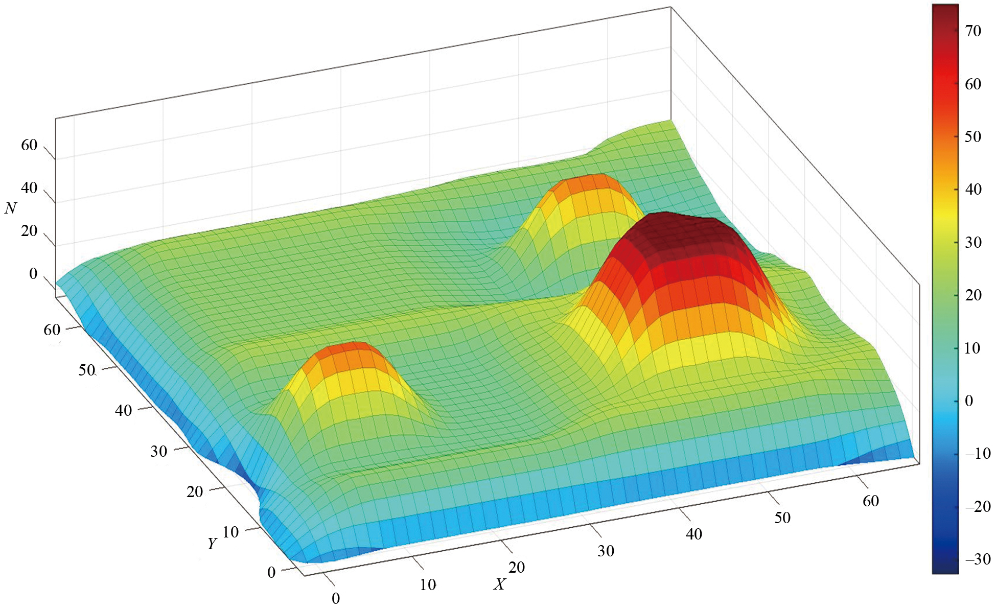
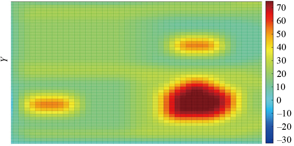
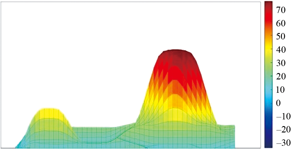
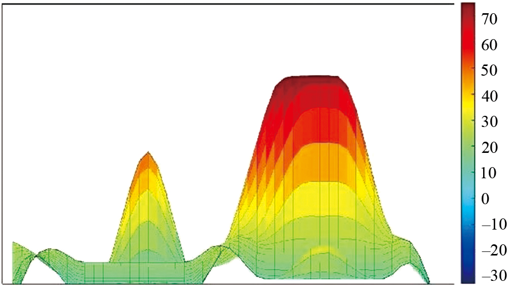
According to the pan-scene energy field construction algorithm proposed in Chapter 3, the energy distribution of this traffic scene is depicted, as shown in Figs. 3 and 4. In this section, the traffic environment, vehicle size, traffic incident and traffic signs are analyzed.
The traffic road shown in Figs. 2 and 5 is a flat road plus slope road. Therefore, it can be seen from the pan-scene energy field distribution shown in Fig. 3 that the energy field state level of the flat road is lower than that of the uphill road and higher than that of the downhill road. However, the overall energy level of the traffic environmental factors is low, which has little impact on the observed objects and can usually be treated as background energy.
The energy distribution law corresponding to the vehicle size is: the energy state value increases with the increase of the vehicle size, and the corresponding threshold interval of the phased collision avoidance area is also wider. Based on the traffic environment, the vehicle model shown in Fig. 3 has a relatively obvious energy distribution according to its size, shape and driving direction, which is usually treated as the foreground field that affects the driving behavior.
Traffic events are formed by stacking temporal effects on the basis of vehicles. In the traffic scene shown in Fig. 3, the traffic time is represented by a two-vehicle rear-end collision instantaneity. At this time, the energy field distribution corresponding to the traffic event is considered as a whole, and the event energy formed by the collision/accident is added based on the energy corresponding to the size of the two vehicles, which affects other traffic participants. Generally, the pan-scene energy formed by the collision event on the driving road is the most obvious, and the driving behavior of the participating traffic participants is also the most affected.
Traffic signs can partly refer to traffic laws and corresponding driving constraints under normal driving behavior, which can be roughly divided into two categories:
(1) Traffic signs on the side of the road, whose influence range is distributed within the observation range of drivers/intelligent driving systems/sensors on the side of the road. In this range, the traffic constraints of the signs will have an impact on the pan-scene energy field;
(2) The shapes of road facilities, such as road markings, railings and zone dividers, also generate interactive energy state distributions, which also act on traffic participants to keep them driving within the allowable lane range.
In the pan-scene system, by the comprehensive effect of the objective traffic scene conditions, the corresponding pan-scene energy distribution will also affect the driving behavior of the observed object. In this paper, we study the longitudinal and lateral dimensions, namely the influence of the energy field distribution on the longitudinal driving speed and the lateral lane change decision.
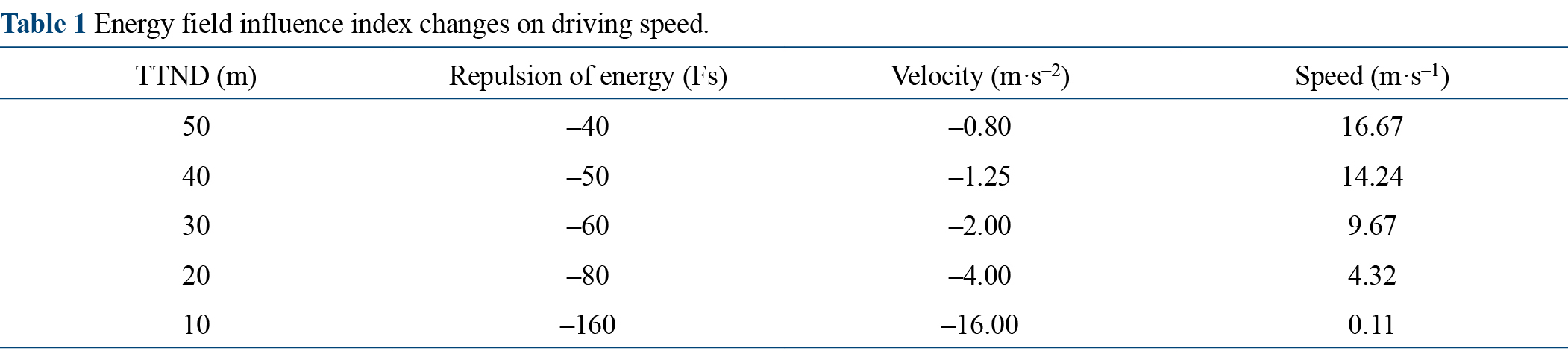
As shown in Fig. 6, in this traffic scene, due to the traffic accident ahead, the corresponding field energy distribution is high, and the influence of energy on the speed of the observer (host vehicle) is strongly related to the urgent time distance of the collision at this time, and the smaller the distance is, the greater the repulsion force of the field will be, and the greater the influence on the speed of the vehicle will be. The influence process can be seen in Table 1. Correspondingly, the car should give priority to slow down driving at this time.
As shown in Fig. 7, due to the traffic accident in front of the observation vehicle, the corresponding lateral energy distribution is high, which produces a large lateral repulsion force for the observation vehicle, which will affect the host vehicle to tend to choose the lane with smaller energy distribution to drive. However, since this scene is set to a single lane, the host vehicle is also subject to the lateral constraint of the traffic sign line, and cannot simply make the lane change choice. Combined with the comprehensive influence of the transverse and longitudinal repulsive forces, the host vehicle in this scenario appears to slow down until it stops. The speed of this scenario as well as the lane change prediction matching metrics are shown in Table 2.
| Scenario | Predictive lane change | Prediction of longitudinal velocity | Root mean suare error (RMSE) |
|---|---|---|---|
| Figure 2 | 0.92 | 0.96 | 0.06 |
In conclusion, the driving pan-scene system based on particle energy filtering can accurately predict and match the driving behavior of the observed objects, which is helpful to comprehensively analyze the development of traffic accidents and guide the driving behavior decision-making of autonomous vehicles.
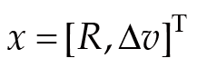
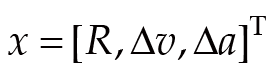
Before the key scene screening work, the scene elements are discretized to build the overall frame ODD of the target scene. Then, since the static scene elements have little influence on the screening process of key scenes, the static scene elements are determined as preset variables before screening [24, 25]. Based on this, the key scenes are screened according to the scene space discretized by the dynamic scene elements. In order to avoid the "dimensional disaster" of the scene, based on the way that the moment when the lane changing center and the lane line coincide as the key moment to cut into and out of the scene, the driving state with the highest importance weight value in the dynamic scene element is selected as the key variable x:(13)where R represents the relative longitudinal distance between the two vehicles at critical moments, that is, the longitudinal distance between the rear bumper of the target vehicle and the front bumper of the host vehicle at the moment when the center of the target vehicle and the lane line coincide, in unit m; Δv represents the change rate of the relative longitudinal distance between two vehicles at critical moments, that is, the relative speed of the target vehicle and the host vehicle when the center of the target vehicle and the lane line coincide, in m·s–1. The range of R is (0,90] m, and the distance is 2 m. The range of Δv is [–20,10] m·s–1, and the distance is 0.4 m·s–1. Thus, R and Δv constitute a two-dimensional scene space, and the number of scenes in the scene space is N(X)=45×76=3420.
At the same time, in order to improve the accuracy of modeling, the driving state quantity is added to the key variable Δa , which represents the change rate of the relative longitudinal distance change rate of the two vehicles at the critical moment, and the unit is m·s–2. In this case, the key variable x for cutting in and out of the scene is:(14)where the range of R is (0,90] m, and the distance is 2 m. The range of Δv is [–20,10] m·s–1, and the distance is 0.4 m·s–1. The range of Δa is [–8,4] m·s–2, and the distance is 0.5 m·s–2. Thus, R, Δv and Δa constitute the 3D scene space, and the number of scenes in the scene space is N(X)=45×76×61=208620.
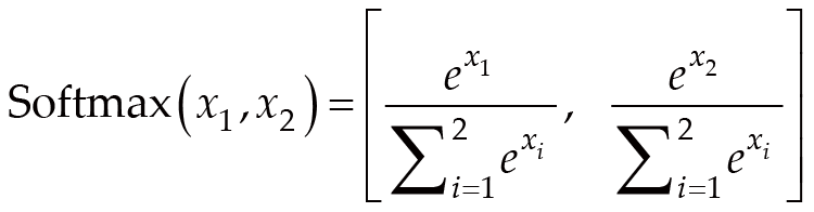
In order to evaluate the scenario risk more comprehensively, the Softmax function in Eq. (15) is introduced, and the comprehensive scenario risk index is obtained by combining the single scenario risk index.(15)
The comprehensive scenario risk index (CRI) can be calculated by(16)
According to the definition of CRI, the higher the value of a single standardized scenario risk indicator, the greater its weight in the comprehensive scenario risk indicator.
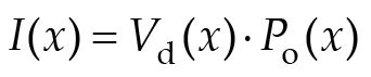
According to the key scene screening criterion, an importance function is designed to represent the importance of the scene [26]. The importance function should consider both the risk of the scene and the occurrence probability of the scene [27]. The scenarios with high risk and high occurrence probability should have higher importance, and a library of important test scenarios should be formed for autonomous vehicle testing. Therefore, the design importance function is as follows.(17)where I(x) is the importance function of the scene, Po(x) is the occurrence probability of the scene, and Vd(x) is the risk degree of the scene.
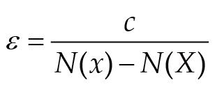
The scenarios that meet the importance threshold will be filtered out and used as key scenarios to form the test scenario library for autonomous vehicle testing [28]. The importance threshold is calculated as follows.(18)where c is a constant greater than or equal to 1, N(x) is the total number of scenes in the scene space, and N(X) is the number of critical scenes [29]. Since the number of critical scenes is generally far less than the total number of scene Spaces, the denominator can be approximately solved according to N(x) when solving the importance threshold.
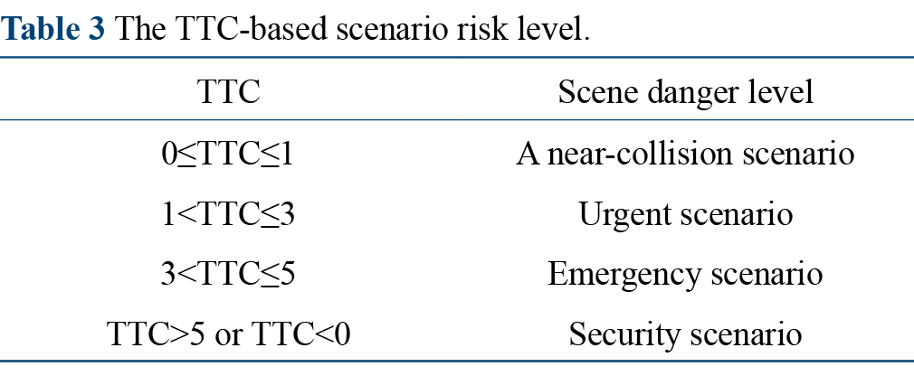
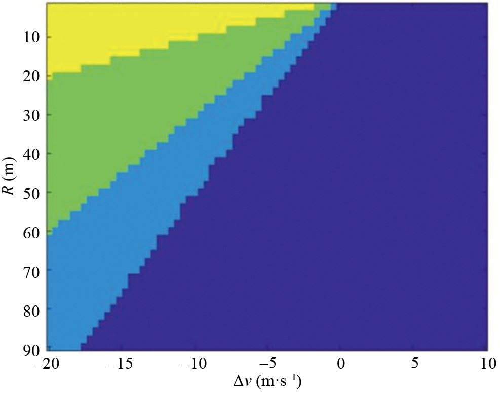
TTC is selected as the evaluation index to evaluate the risk degree of the scene in the two-dimensional scene space. Table 3 shows the TTC-based hazard level classification method for the scene. Specifically, the scene with TTC greater than 0 s and less than or equal to 1 s is divided into the scene on the verge of collision, and the scene hazard is set to 1. The scenarios with ETTC greater than 1 s and less than or equal to 3 s were divided into urgent scenarios, and the risk of the scenario was set to 0.7. The scenarios with ETTC greater than 3 s and less than or equal to 5 s were divided into emergency scenarios, and the risk of the scenario was set to 0.4. The scenarios with ETTC greater than 5 s are classified as safe scenarios, and the scenario hazard is set to 0. The scene hazard level diagram is shown in Fig. 8.
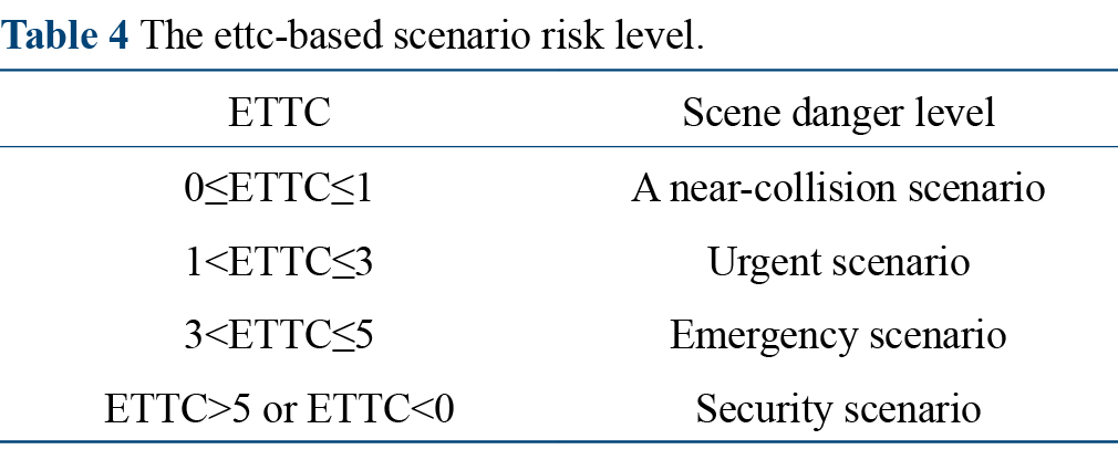
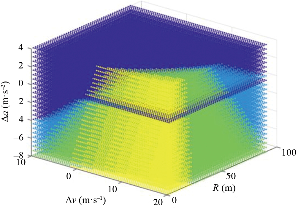
ETTC is selected as the evaluation index to evaluate the risk degree of the scene in the 3D scene space [30]. The classification method of scene danger level based on ETTC is shown in Table 4. Specifically, the scene with ETTC greater than 0 s and less than or equal to 1 s is divided into the scene on the verge of collision, and the scene hazard is set to 1. The scenarios with ETTC greater than 1 s and less than or equal to 3 s were divided into urgent scenarios, and the risk of the scenario was set to 0.7. The scenarios with ETTC greater than 3 s and less than or equal to 5 s were divided into emergency scenarios, and the risk of the scenario was set to 0.4. The scenarios with ETTC greater than 5 s are classified as safe scenarios, and the scenario hazard is set to 0. The scene hazard level diagram is shown in Fig. 9.
The natural driving database provided by China Automotive Technology Research Center is used to solve the scene occurrence probability [31]. Among them, the data of the database is calibrated by watching the video to determine the scene type and the vehicle type in the scene [32]. According to the ODD designed in this paper, the left cut in scene, right cut in scene, left cut out scene and right cut out scene are extracted from the natural driving database, and the real scene in the natural driving database is transformed into the scene in the scene space obtained by the discretization of the scene elements by using the convex combination method, so as to obtain the occurrence probability of the scene in the scene space.
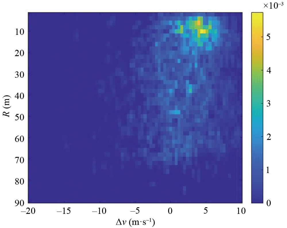
After screening, a total of 6364 cases of left-cut scenes were extracted from the natural driving database, and the scene probability of the left-cut scene in the two-dimensional scene space was calculated, and the calculation results are shown in Fig. 10. It can be seen from the figure that in the scene of left cut on the real road, the relative speed distribution of the two vehicles is relatively concentrated, mainly distributed in the interval of [–4,8] m·s–1. The distribution of the relative distance between the two vehicles is relatively scattered, and it is distributed in the interval range of [2, 70] m. In all the scenarios, the region with the highest probability of scene occurrence is concentrated in the range of the relative speed interval of the two vehicles is [–1,5] m·s–1, and the relative distance interval of the two vehicles is [2, 16] m.
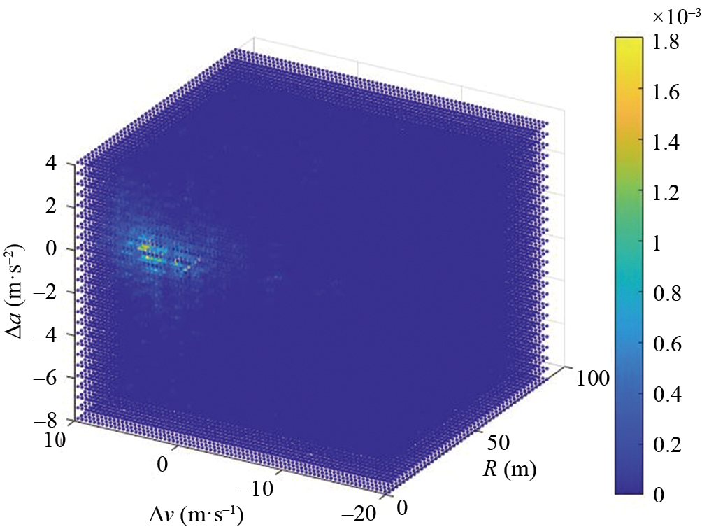
The scene probability of the left cut-in scene in the 3D scene space is calculated, and the calculated results are shown in Fig. 11. There are 208,620 discrete scenes in the 3D scene space, which is a huge number of scenes. It can be seen from the figure that after considering the relative speed and distance of the two vehicles and adding the relative acceleration of the two vehicles, the scene occurrence probability of the left-cut scenario on the real road is still concentrated in a relatively small area. Increasing the relative acceleration of two vehicles does not affect the distribution of the relative velocity and the relative distance of two vehicles. The high probability distribution interval of the relative velocity and the relative distance of two vehicles is the same as that of the two-dimensional scene space, and the relative acceleration of two vehicles is concentrated between [–1,1] m·s–2. The relative acceleration interval of the two vehicles in the scenario with high occurrence probability is [–1/2,1/2] m·s–2.
After screening, a total of 9679 cases of right-cut scenes were extracted from the natural driving database, and the scene probability of right-cut scenes in the two-dimensional scene space was calculated, and the calculation results are shown in Fig. 12. It can be seen from the figure that in the right-cut scene on the real road, the relative speed distribution of the two vehicles is relatively concentrated, mainly distributed in the interval of [–5, 8] m·s–1. The distribution of the relative distance between the two vehicles is relatively scattered, and it is distributed in the interval range of [2,72] m. In all the scenarios, the region with the highest probability of scene occurrence is concentrated in the range of the relative speed interval of the two vehicles is [2,5] m·s–1, and the relative distance interval of the two vehicles is [4,12] m.
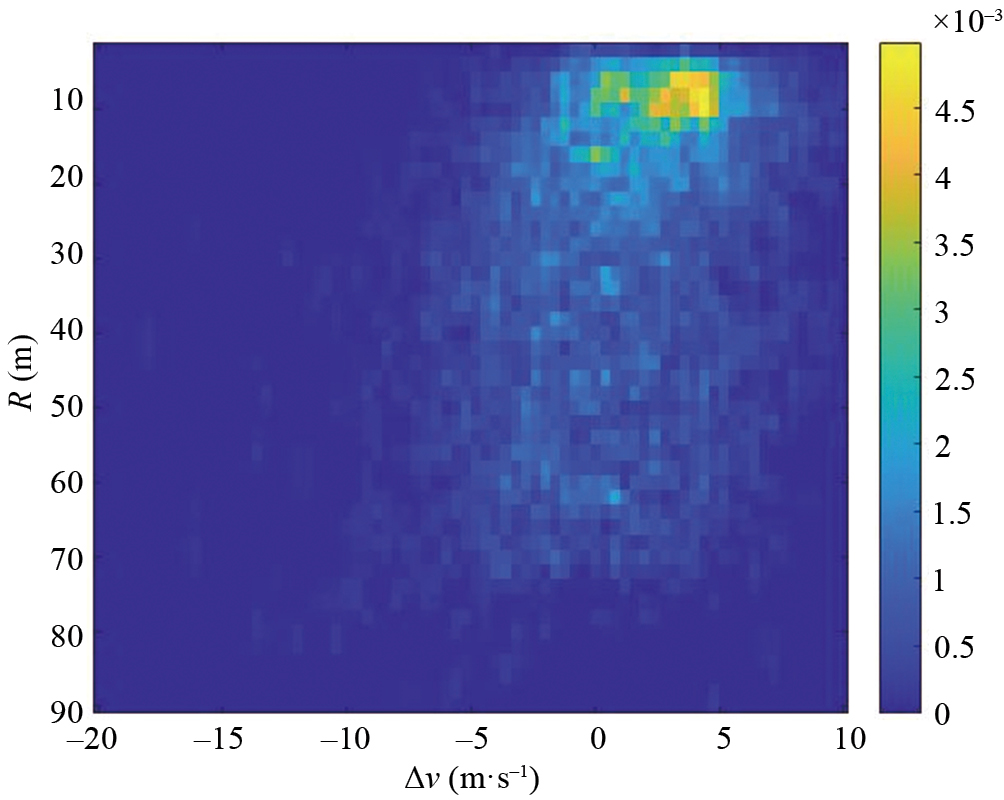
The scene probability of the right-cut scene in the 3D scene space is calculated, and the calculated results are shown in Fig. 13. It can be seen from the figure that after considering the relative speed and distance of two vehicles and adding the relative acceleration of two vehicles, the scene occurrence probability of the right-cut scene on the real road is still concentrated in a relatively small area. Increasing the relative acceleration of two vehicles will not affect the independent distribution of the relative velocity and the relative distance of two vehicles. The high probability distribution interval of the relative velocity and the relative distance of two vehicles is the same as that of the two-dimensional scene space, and the relative acceleration of two vehicles is concentrated between [–1/2,3/2] m·s–2. The relative acceleration interval of the two vehicles in the scenario with high occurrence probability is [0,1] m·s–2.
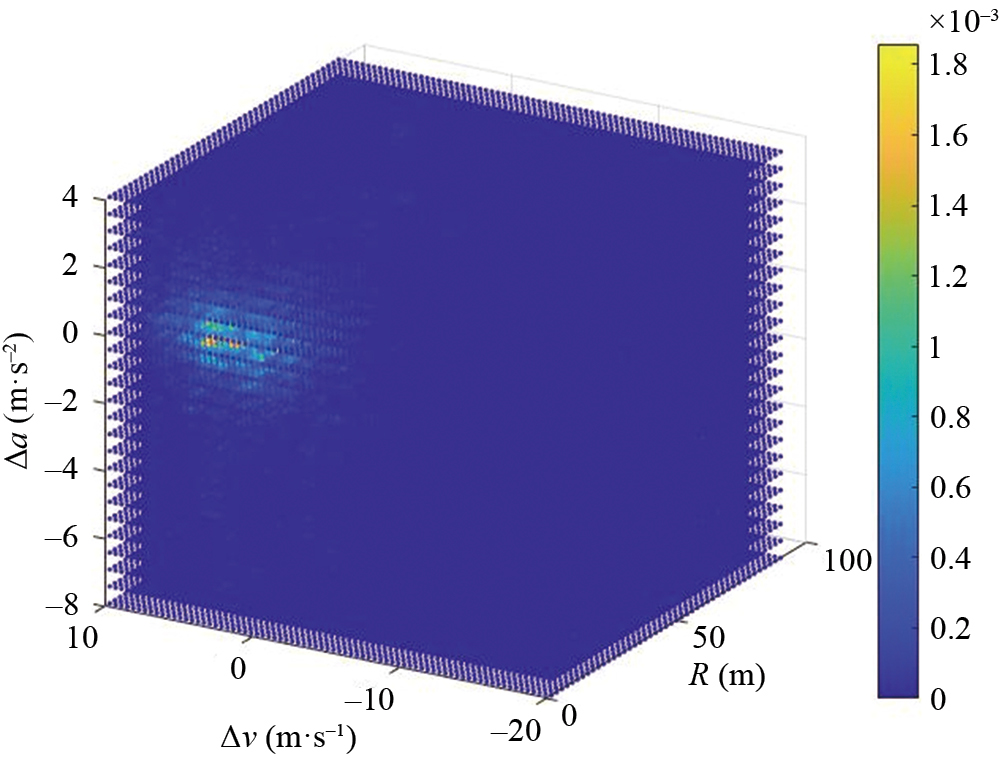
In summary, by comparing the scene occurrence probability distribution of the left cut scene and the right cut scene in the 2D scene space and the 3D scene space, it can be seen that the concentrated area of the scene occurrence probability of the left cut scene and the right cut scene is roughly consistent with the high occurrence probability area because they both belong to the scene type of the cut scene. However, the different entry directions will also cause figslight changes between the concentrated area and the high probability area, which may be caused by the differences in drivers' perspective and driving habits under the two entry modes brought by the driver's position on the left side of the vehicle in China.
After screening, a total of 3128 cases of left cut out scenarios were extracted from the natural driving database, and the scene probability of left cut out scenarios in the two-dimensional scene space was calculated, and the calculation results are shown in Fig. 14. It can be seen from the figure that in the scene of left cut out on the real road, the relative speed distribution of the two vehicles is relatively scattered, which is distributed in the interval of [–20,10] m·s–1, and the distribution is relatively concentrated in the interval of [–4,7] m·s–1. The distribution of the relative distance between the two vehicles is also of (0,70] m. In all the scenarios, the area with the highest probability of scene occurrence is mainly concentrated in the range of the relative speed interval of the two vehicles is [–1,3] m·s–1 and the relative distance interval of the two vehicles is [8, 16] m. In addition, there are scattered distributions in several other inter-cell segments.
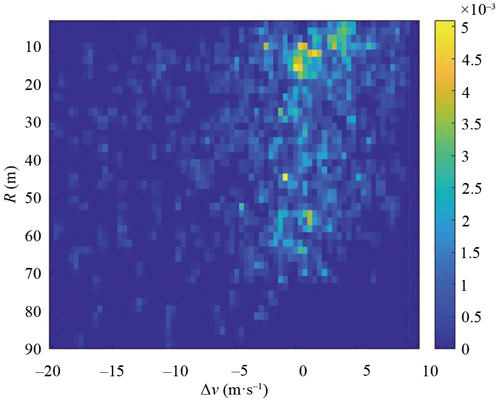
The scene probability of the left cut out scene in the 3D scene space is calculated, and the calculated results are shown in Fig. 15. As can be seen from the figure, after considering the relative speed and distance of two vehicles and adding the relative acceleration of two vehicles, the scene occurrence probability of the left-cut scene on the real road becomes concentrated, which is caused by the fact that the total number of scenes in the three-dimensional scene space (208,620) is much larger than that in the two-dimensional scene space (3420). Although increasing the relative acceleration of two vehicles does not affect the independent distribution of the relative velocity and the relative distance of two vehicles, the distribution of the scene in the concentrated area becomes more uniform in the whole 3D scene space. The high probability distribution interval of the relative speed and the relative distance of the two vehicles are the same as the high probability distribution interval in the two-dimensional scene space, and the relative acceleration of the two vehicles is concentrated between [–1/2, 3/2] m·s–2.
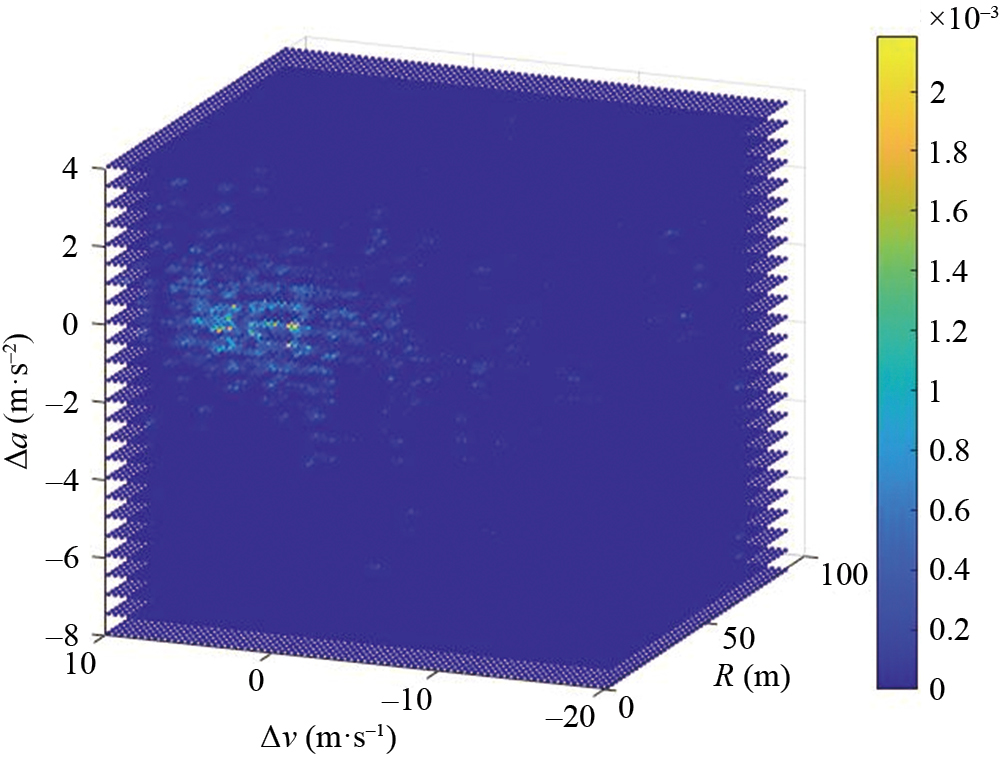
Comparing cut-in scene and cut-out scene, it can be found that there are obvious differences in scene occurrence probability distribution between them, whether in 2D scene space or 3D scene space. This is because cut-out scene and cut-out scene belong to two completely different scene types, scene structure and scene characteristics. By analyzing the differences between the two, it can be found that the occurrence probability distribution of the cut-in scene is relatively concentrated and the internal regularity is strong, while the occurrence probability distribution of the cut-out scene is scattered and the internal regularity is weak, which is consistent with the scene characteristics of the cut-in scene and cut-out scene. A considerable part of the cut-in scene needs to overtake the vehicle first and then start cutting. Moreover, the cutting process can only be observed through the rear view mirror, and the overall dangerous degree of the scene is high. Therefore, the operation of both the cutting vehicle and the host vehicle in the cutting process will be more careful to ensure that the vehicle is always in the safety zone as much as possible. The completion of the cut-out scene does not need to take overtaking as the premise, and there is no requirement for the relative distance between the two vehicles. Except for the emergency condition, most of the host vehicles will choose to cut out under the condition of a large relative distance between the two vehicles, and the overall risk of the scene is small, so the scene distribution is scattered.
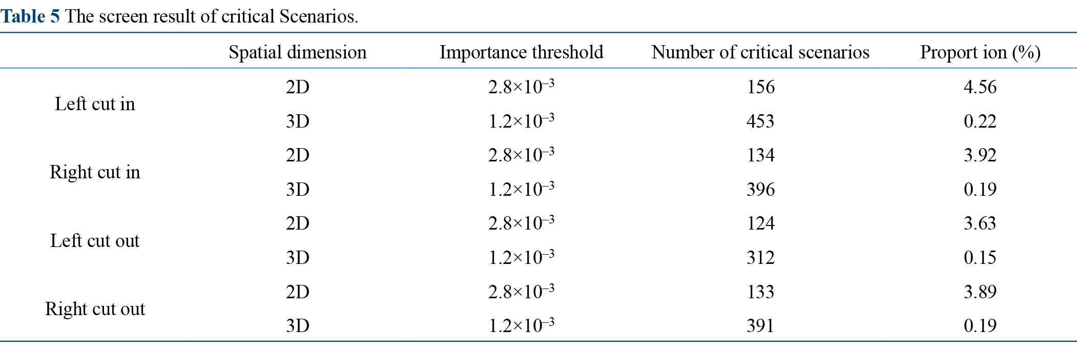
Based on the calculation results of the above scenario risk degree and scenario occurrence probability, the importance function value of the scenario is calculated according to Eqs. (17) and (18). The scenarios that meet the threshold of the importance function will be screened out and used as key scenarios to form a test scenario library for autonomous vehicle testing. In the screening of critical scenes, due to the large number of scenes in the scene space, in order to speed up the search efficiency of critical scenes, two optimization algorithms, multi-start optimization algorithm and flooding filling algorithm, are used to search for critical scenes. The screening results are shown in Table 5.
As can be seen from the screening results in Table 5, in the 2D scene space and 3D scene space, the key scenes that cut into the scene and cut out the scene account for a small proportion of the total number of scenes, both less than 5%, indicating that in the scene space, the number of scenes with a large degree of danger and a certain probability of occurrence on the real road is small. Whether the scene is cut into or out of the scene, the proportion of the key scenes in the 3D scene space is much smaller than that in the 2D scene space. The proportion of the key scenes in the 2D scene space is between 3%–5%, and the proportion of the key scenes in the 3D scene space is within 0.3%, which indicates that the total number of scenes increases exponentially with the increase of the dimension of the scene space. But the number of critical scenarios grows is relatively small.
The above results show that a small proportion of the key scenes with regard to the scene space is successfully obtained through the key scene screening theory. Applying these key scenes to the test of autonomous driving vehicles will significantly improve the test efficiency and accelerate the test process. Therefore, this method has stronger practical significance than the traditional scene screening that only considers the risk. Comparing the number of key scenes between cut-in scene and cut-out scene, the number of key scenes between cut-in scene and cut-out scene is the largest, and the number of key scenes between cut-in scene and cut-out scene is the least. However, on the whole, the number of key scenes between cut-in scene and cut-out scene in two-dimensional scene space and three-dimensional scene space is roughly the same. It shows that although the distribution of the occurrence probability of the cut-in scenario and the cut-out scenario is different, it does not significantly affect the importance function value of the scene. The reason is that although the probability distribution of the cut-out scenario is scattered, and there are many scenarios with high occurrence probability, most of the scenarios with high occurrence probability have low risk, so the importance function value is still small. Therefore, there is no increase in the critical scene of the cut out scene.
According to the theory of key scene generation, the key scene generated by the cut-in scene and cut-out scene should be a scene with high danger and a certain probability of occurrence on the real road. Therefore, the scenario risk of the obtained critical scenarios is verified by the scenario risk assessment method proposed above.
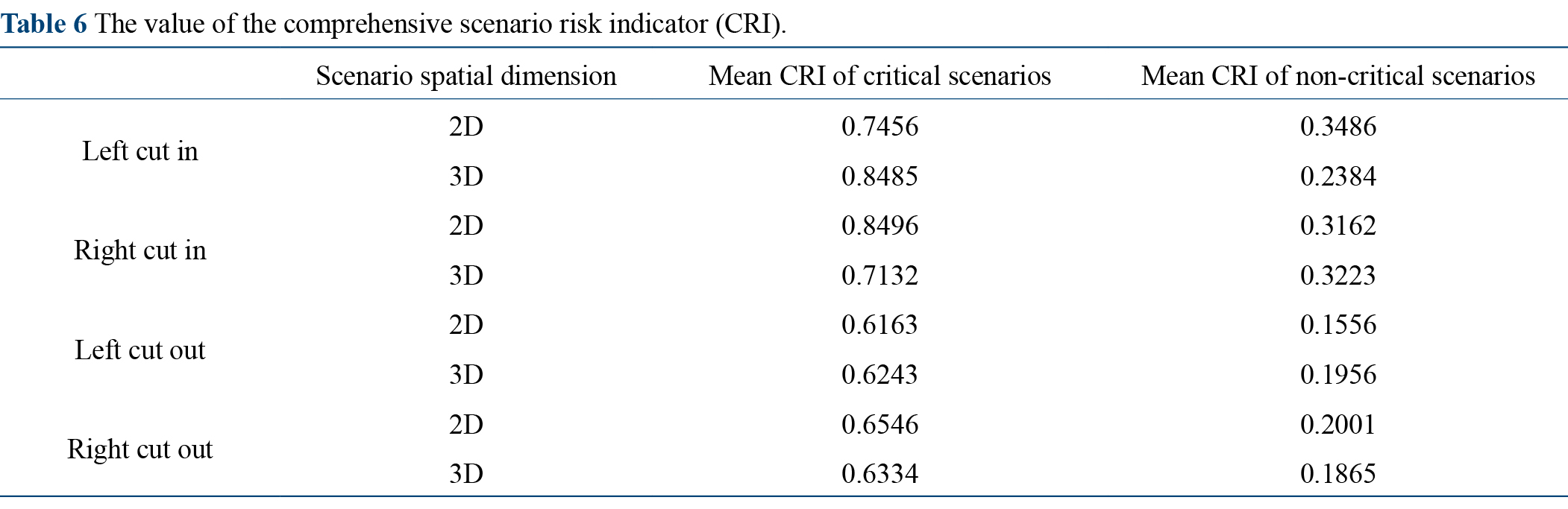
By sampling, 50 key scenes are randomly selected from the two-dimensional key scenes of the cut-in scene and cut-out scene, and the comprehensive scene risk index is calculated. At the same time, 50 critical scenes are randomly selected from the non-critical scenes in the corresponding two-dimensional scene space, and the comprehensive scene risk index is calculated as a control. Similarly, 150 key scenes are randomly selected from the 3D key scenes of the cut-in scene and cut-out scene, and the comprehensive scene risk index is calculated. At the same time, 150 key scenes are randomly selected from the non-key scenes of the corresponding 3D scene space, and the comprehensive scene risk index is calculated as a control. The calculation results are shown in Table 6.
It can be seen from the table that the mean value of the comprehensive scene risk index of the critical scene is greater than that of the non-critical scene in the two-dimensional scene space and three-dimensional scene space, regardless of the cut-in scene and cut-out scene, the mean value of the comprehensive scene risk index of the critical scene is above 0.6, and the mean value of the CRI of the non-critical scene is below 0.35. It shows that the critical scenes generated by the critical scene screening theory are indeed scenes with high risk, which proves the effectiveness of the critical scene screening theory. By observing the mean value of the comprehensive scene risk index of non-critical scenes, it can be seen that non-critical scenes also have a certain scene risk. This is because when selecting key scenes through the critical scene generation theory, some scenes with a certain risk degree but a low probability of happening on the real road are discarded. However, since the number of this part of scenarios is small and most of the non-critical scenarios in the scenario space are security scenarios, the mean value of the overall comprehensive scenario risk index is small.
Based on the construction of the pan-scene system, this paper applies the particle energy filter to model the pan-scene energy change, and then establishes the intelligent driving strategy rules and the scene energy evaluation index. Through the simulation data verification, the comprehensive energy of the pan-scene system and the energy change caused by the superposition event are described and verified. And the key scenes are screened and analyzed based on the scene danger classification table of ETTC. The experimental results show that in the complex scene considering the interaction of traffic participants, the repulsive force caused by chain risk events and the comprehensive action field of the traffic destination are consistent with the traffic strategy and driving behavior. The matching indexes of the predicted steering and longitudinal speed are 0.92 and 0.96, respectively, and the average root mean square error is 0.06. The proposed method can improve the safety and comfort of the system, reduce the sharp shock of the field and overcome the excitation of dangerous events, so as to improve the practicability of the automatic driving system in the superimposed dangerous field.
In the future work, the influence of multi-observation means on the pan-scene particle system will be considered under more complex conditions, such as weather, other risk events such as temporary road facilities change, and multi-sensor perception fusion system under high-precision map, so as to carry out theoretical optimization and practical iteration, and further explore the real-time multi-dimensional scene evaluation under the pan-scene system.
PEGASUS, "PEGASUS expert worshop #1,"2016, Accessed on June, 2024. [Online] Available: https://www.vvm-projekt.de/en/news-events.
UNECE, "Working party on automated/autonomous and connected vehicles – Introduction,"Accessed on June, 2024. [Online] Available: https://unece.org/transport/vehicle-regulations/working-party-automatedautonomous-and-connected-vehicles-introduction, 2020.
ASAM, "ASAM SIM: Guide, Standardization for highly automated driving,"2021, Accessed on June, 2024. [Online] Available: https://www.asam.net/asam-guide/.
O. Khabit, "Real-time obstacle avoidance for manipulators and mobile robots," The International Journal of Robotics Research, vol. 5, no. 2, pp. 500–505, 1986.
F. Anhalt and S. Hafner, "Concept, implementation, and performance comparison of a particle filter for accurate vehicle localization using road profile data," SAE International Journal of Vehicle Dynamics, Stability, and NVH, vol. 7, no. 3, pp. 405–418, 2023.
G. Y. Chen, J. Yao, Z. H. Gao, Z. Gao, X. M. Zhao, and N. Xu, "Emergency obstacle avoidance trajectory planning method of intelligent vehicles based on improved hybrid A*," SAE International Journal of Vehicle Dynamics, Stability, and NVH, vol. 8, no. 1, pp. 3–19, 2024.
Y. Wang, H. G. Wei, L. Yang, and B. B. Hu, "A review of dynamic state estimation for the neighborhood system of connected vehicles," SAE International Journal of Vehicle Dynamics, Stability, and NVH, vol. 7, no. 3, pp. 367–385, 2023.
D. Gonzalez, J. Perez, V. Milanés, and F. Nashashibi, "A review of motion planning techniques for automated vehicle," IEEE Transactions on Intelligent Transportation Systems, vol. 17, no. 4, pp. 1135–1145, 2016.
S. Ge and Y. Cui, "Dynamic motion planning for mobile robots using potential field method," Autonomous Robots, vol. 13, pp. 207–222, 2002.
A. Einstein, "Unified field theory based on riemannian metrics and distance parallelism," Math Annal, vol. 102, pp. 685–697, 1930.
J. Ji, H. Peng, W. Chi, and M. Tang, "Decision making for vehicle collision avoidance based on dangerous potential field,"in Proceedings of 2015 Annual Meeting of China Automotive Engineering Society, Shanghai, China SAE, 2015.
Y. Ren, L. Zheng, W. Zhang, W. Yang, and Z. B. Xiong, "A study on active collision avoidance control of autonomous vehicles based on model predictive control," Automotive Engineering, vol. 41, no. 4, pp. 404–410, 2019.
C. Xiu and H. Chen, "Research on local path planning of unmanned vehicle based on improved artificial potential field method," Automotive Engineering, vol. 35, no. 9, pp. 808–811, 2013.
K. Lewin, "Field theory in social science," American Catholic Sociological Review, vol. 12, no. 2, p. 103, 1951.
ISO, International standard ISO 21448: 2022, "Road vehicles — Safety of the intended functionality," 2022, Accessed on June, 2024. [Online] Available: https://www.iso.org/standard/70939.html.
S. Ulbrich, T. Menzel, A. Reschka, F. Schuldt, and M. Maurer, "Defining and substantiating the terms scene,situation, and scenario for automated driving,"2015 IEEE 18th International Conference on Intelligent Transportation Systems, Gran Canaria, Spain, 15–18 September, 2015.
Y. Hu, M. Dai, K. Wang, and L. Drugge, "Cut-in critical level prediction via simulation based time-to-collision algorithm,"2020 25th IEEE International Conference on Emerging Technologies and Factory Automation (ETFA), Vienna, Austria, 08–11 September, 2020.
J. Ren, C. Yu, S. Sheng, X. Ma, H. Zhao, S. Yi, and H. Li, "Balanced meta-softmax for long-tailed visual recognition," arXiv:2007.10740 [cs.LG], 22 November, 2020.
M. Hayat, S. Khan, S. W. Zamir, J. Shen, and L. Shao, "Gaussian affinity for max-margin class imbalanced learning,"2019 IEEE/CVF International Conference on Computer Vision (ICCV), Seoul, Korea (South), 27 February, 2020, pp. 6468–6478.
S. H. Khan, M. Hayat, M. Bennamoun, F. A. Sohel, and R. Togneri, "Cost-sensitive learning of deep feature representations from imbalanced data," IEEE Transactions on Neural Networks and Learning Systems, vol. 29, no. 8 pp. 3573–3587, 2018.
P. Wang, K. Han, X.-S. Wei, L. Zhang, and L. Wang, "Contrastive learning based hybrid networks for long-tailed image classification, 2021 IEEE/CVF Conference on Computer Vision and Pattern Recognition (CVPR), Nashville, TN, USA, 20–25 June, 2021, pp. 943–952.
Q. Dong, S. Gong, and X. Zhu, "Class rectification hard mining for imbalanced deep learning," arXiv:1712.03162 [cs.CV], 8 Dec 2017.
T.-Y. Lin, P. Goyal, R. Girshick, K. He, and P. Dollár, "Focal loss for dense object detection,"2017 IEEE International Conference on Computer Vision (ICCV), Venice, Italy, 22–29 October, 2017, pp. 2999–3007.
D. Mahajan, R. Girshick, V. Ramanathan, K. He, M. Paluri, Y. Li, A. Bharambe, and L. Van Der Maaten, "Exploring the limits of weakly supervised pretraining," arXiv:1805.00932 [cs.CV], 2 May 2018.
Y. Cui, Y. Song, C. Sun, A. Howard, and S. Belongie, "Large scale fine-grained categorization and domain-specific transfer learning," arXiv:1806.06193 [cs.CV], 16 Jun, 2018.
B. Kang, S. Xie, M. Rohrbach, Z. Yan, A. Gordo, J. Feng, and Y. Kalantidis, "Decoupling representation and classifier for long-tailed recognition," arXiv:1910.09217 [cs.CV], 19 February, 2020.
B. Zhou, Q. Cui, X. Wei, and Z.-M. Chen, "BBN: Bilateral-branch network with cumulative learning for long-tailed visual recognition," arXiv:1912.02413 [cs.CV], 10 March, 2020.
P. Chu, X. Bian, S. Liu, and H. Ling, "Feature space augmentation for long-tailed data," arXiv:2008.03673 [cs.CV], 9 August, 2020.
J. Liu, Y. Sun, C. Han, Z. Dou, and W. Li, "Deep representation learning on long-tailed data: A learnable embedding augmentation perspective,"2020 IEEE/CVF Conference on Computer Vision and Pattern Recognition (CVPR), Seattle, WA, USA, 13–19 June, 2020, pp. 2967–2976.
J. Kim, J. Jeong, and J. Shin, "M2m: Imbalanced classification via major-to-minor translation," arXiv:2004.00431, 20 December, 2020.
S. S. Mullick, S. Datta, and S. Das, "Generative adversarial minority oversampling,"2019 IEEE/CVF International Conference on Computer Vision (ICCV), Seoul, Korea (South), 27 October, 2019, pp. 1695–1704.
H. Zhang, M. Cisse, Y. N. Dauphin, and D. Lopez-Paz, "mixup: Beyond empirical risk minimization," arXiv:1710.09412 [cs.LG], 27 Apr 2018.
 Top
Top