ContentsFigures & Tables
With the rapid socioeconomic development, the number of vehicles has grown rapidly, which has brought about many negative problems such as traffic accidents, traffic congestion, and environmental pollution [1]. Vehicle formation is a potential solution to these problems, enabling vehicles to adjust their longitudinal motion according to the state of neighboring vehicles to achieve a consistent speed of vehicles inside the platoon and obtain the desired vehicle spacing [2]. Since all vehicles in the platoon are in a similar state, this improves efficiency, fuel economy, and driving safety [3].
Predictive cruise control (PCC) is a method that uses predictive information (e.g., forward-looking information about road gradients, the phase and timing of upcoming traffic signals, and the movement status and trends of surrounding vehicles) to construct an optimal control problem and determine the optimal driving strategy [4]. The highway is a typical scenario of vehicle driving, and PCC in this scenario mainly uses the forward-looking information of road slope to plan the economic speed of the vehicle and improve fuel economy. Lattemann et al. [5] constructed the PCC algorithm with the optimization objective of minimizing fuel consumption based on the road slope information, and the simulation results proved that the algorithm can improve the fuel economy of vehicles. Chu et al. [6] constructed a PCC problem based on model predictive control (MPC) using slope information from a high-definition map, and the average fuel saving of the proposed algorithm was 8.73% by comparing it with adaptive cruise control (ACC) in a real experiment. To further exploit the energy-saving potential of the platoon, some scholars have combined the platoon with PCC. Turri et al. [7] designed a hierarchical framework where the upper layer is based on dynamic programming (DP) to calculate the platoon economic speed profile and the lower layer is based on distributed model predictive control (DMPC) to track the planned speed, which was experimentally shown to achieve 12% fuel saving. Zhai et al. [8] proposed an ecological cooperative look-ahead control problem formulated based on DMPC and designed a particle swarm optimization algorithm with multiple dynamic populations (PSO-MDP) to quickly solve the Eco-CLC. Most of the current research on PCC of platoon assumes that there are no ambient vehicles on the road and only focuses on the longitudinal speed planning of the platoon. However, during the actual driving of the platoon, there are bound to be ambient vehicles on the road, which can lead to the unguaranteed enforceability of the speed planning results, such as the scene where the speed of the preceding vehicle is lower than the planned speed. If the platoon cannot change lanes, it will force the PCC system to exit, which not only requires additional personnel to take over but also disrupts the continuity of the platoon's operation [9]. If predictive cruise control of platoon can consider lane changing, it can provide a new dimension and more possibilities for speed planning [10], which can safely improve the efficiency and economy of platoon driving.
Lane change is a basic behavior of vehicle driving, which is more complex compared to car-following, and has higher requirements for decision-making, planning, and control. At present, there are few studies on platoon lane change (PLC) maneuvers, mainly focusing on single vehicle lane change. The approaches to lane change decision-making of single vehicle can be divided into four categories, including rule model, utility function model, data-driven model, and game theory model. The rule model requires human-designed rules to judge the behavior that a vehicle should take, and the more common rule models include decision trees [11] and state machines [12]. The utility function model requires a cost function to make decisions based on costs. Nilsson et al. [13] designed a utility function that expresses the utility of each lane relative to time and allows for simultaneous consideration of mandatory, discretionary, and anticipatory lane change decisions. Feng et al. [14] designed a local cost map that contains road costs, traffic costs, and arrival costs, and used breadth-first search (BFS) to find the minimum cost. The data-driven model can learn lane change strategies from a large amount of lane change data, and common approaches package deep learning (DL) [15] and reinforcement learning (RL) [16]. The game theoretic model can describe the competitive and cooperative relationships between lane change vehicles and other traffic participants, and are a current research hotspot. Zhang et al. [17] came up with a game theoretic model with aggressiveness estimation, which can continuously establish a game with candidate vehicles, evaluate the aggressiveness of the candidate vehicles through the interactions between vehicles, and select the behavior with the highest gain. Wang et al. [18] proposed a lane change strategy based on harmonious deep reinforcement learning, where the intelligences exchange their respective strategies after each round of learning and eventually reach a zero-sum game state. Most of the current lane change decision models focus only on the instantaneous gain of the target vehicle after the lane change [16], without considering that the value judgment of the lane change decision-making is also affected by the future traffic conditions. For example, even though the target vehicle can gain faster driving speed or bigger driving space in the instant after lane change, it may be blocked by new slower vehicles in the target lane after a period of time. If the lane change decision-making model can take future driving conditions into account, it helps the target vehicle to gain longer-term benefits.
PCC of platoon and lane change decision-making models require a wealth of predictive information, and the cloud can provide wide-area dynamic traffic information to more accurately predict future driving conditions and improve the foresight of decision-making and planning. K. Li et al. [19, 20] proposed a cloud control system (CCS) based on a new generation of mobile connected technology, which can achieve the improvement of comprehensive performance of vehicles and traffic systems by integrating sensing, decision-making and control, and the related technology has been initially validated. Zhao et al. [21] proposed a CCS-based platooning centralized MPC algorithm, which was deployed on the edge cloud, and analyzed the impact of vehicle cloud communication delay on platoon control. S. Li et al. [22] designed a CCS-based PCC hierarchical algorithm, which was deployed on the edge cloud, to calculate the economic speed and gear and dispatched to vehicles. Simulation results show that the algorithm saves about 6.17% fuel relative to constant cruise. Gao et al. [23] studied a continuous signal intersection scenario for an urban bus, and based on the cloud control system to obtain traffic signal status and traffic conditions, designed a queueing time prediction model and planned the optimal speed through the DP algorithm, which enabled the vehicle to pass through the continuous intersection without stopping to achieve about 50% energy saving. CCS allows the target vehicle to establish connections with environmental vehicles, roadside infrastructure, and cloud control platforms and can provide wide-area dynamic traffic information for target vehicles to better predict upcoming events, enabling vehicles to predictably adjust their driving strategies and obtain comprehensive performance improvements in terms of safety, efficiency, and economy. In addition, the algorithm can be deployed on a low-latency edge cloud to reduce the computational burden of vehicles and achieve efficient utilization of computational resources.
In this study, we propose a CPPLC system in highway scenarios. Specifically, first, a vehicle-cloud hierarchical control architecture for CPPLC is proposed under the general architecture of CCS. Then, the predictive lane-changing decision-making (PPLD) algorithm deployed in the cloud is designed to collaboratively optimize the platoon longitudinal acceleration and lateral lane-changing decision-making. Finally, the trajectory planner and tracking controller on the vehicle are designed to track the commands given by the cloud. The main contributions of this study are summarized as follows:
(1) The vehicle-cloud hierarchical control architecture of CPPLC system is proposed. In this architecture, CCS and platoon form a rolling closed-loop control.
(2) The PPLD algorithm is designed. The real-time state and future change trend of vehicles in the environment around the platoon are taken as the a priori information, the longitudinal acceleration and lateral lane-changing decision of the platoon are taken as the decision quantities to construct the optimal control problem, and a hierarchical solution strategy is designed to realize the fast solution of the optimization problem.
The structure of this paper is as follows. Section 2 designs the vehicle-cloud hierarchical control architecture for the CPPLC system and introduces the model of vehicles used in this paper. Section 3 describes the PPLD algorithm in the cloud. Section 4 presents the trajectory planning algorithm and distributed platoon controller on the vehicle. Simulation experiments are designed and the simulation results are analyzed in Section 5. Section 6 provides a summary and outlook.
CCS can overcome the limitations of communication distance and sensing range of single-vehicle autonomous driving. This section first introduces CCS, then designs the vehicle cloud hierarchical control architecture of CPPLC based on the general architecture of CCS, and introduces the components of the algorithm, and finally introduces the dynamics model and fuel consumption model of the vehicle used in this paper.
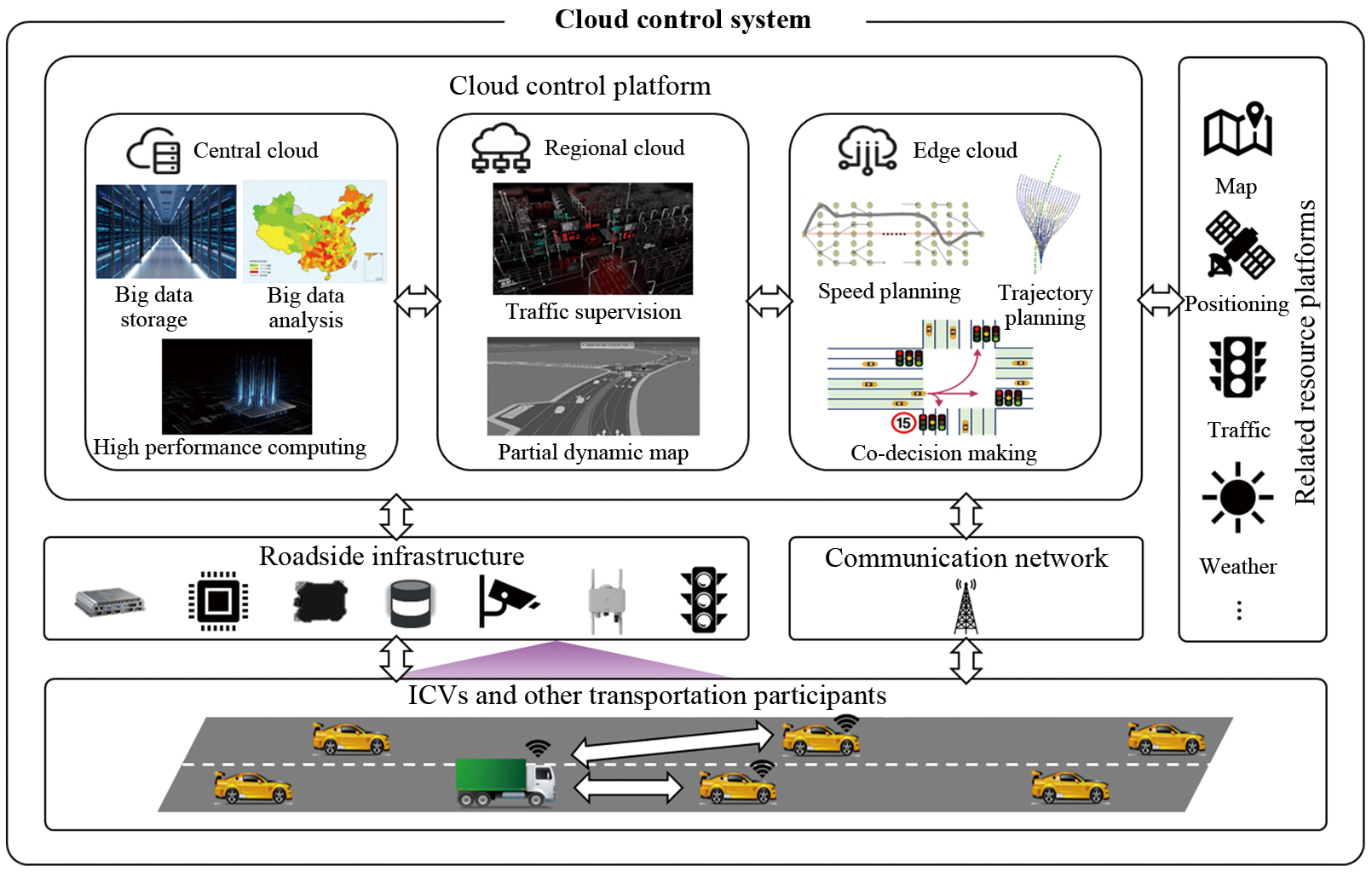
CCS is the abbreviation of the coordinated control system by vehicle-road-cloud integration, which is an integrated system for intelligent connected vehicles (ICVs) and transportation with the cloud control platform (CCP) as the core. The system consists of the CCP, roadside infrastructure, ICV, communication network, and related resource platform [19, 20]. The overall architecture of CCS is shown in Fig. 1.
The CCP is composed of a cloud control base platform and a cloud control application platform. Among them, the cloud control infrastructure platform is the core of CCP, which integrates the dynamic information of ICVs, roadside infrastructure, and related resource platforms to provide basic services for vehicles and related sectors. According to the real-time requirements and service scope requirements, the cloud control infrastructure platform can be divided into edge cloud, regional cloud, and central cloud. The edge cloud is the closest level to the vehicle road, providing real-time computing services for ICVs. Regional clouds are aggregations of multiple edge clouds that provide weak real-time and non-real-time computing services for transportation and management. The central cloud is the convergence of multiple regional clouds, providing macro traffic data analysis and value-added data services. Three levels of clouds work together to support different service requirements. Cloud control application platform is a collection of all kinds of applications realized under the support of the CCS system, including intelligent driving applications to improve the performance of a single vehicle, intelligent transportation applications to improve traffic efficiency and traffic big data applications, etc., to provide differentiated application services for various customers.
ICVs are the direct data source as well as control and service object of the CCS, sharing data with the CCP, roadside infrastructure, and other ICVs through the communication network, and receiving control commands from the CCP to realize the optimization and improvement of the overall performance of single vehicles and regional traffic.
CCS has five main features: vehicle-road-cloud interconnection, digital mapping of traffic elements, global performance optimization, efficient computation and scheduling, and high reliability [19, 20]. It helps the vehicle to obtain the actual road conditions and traffic conditions on the subsequent road and calculate the best driving strategy, which in turn improves the driving performance of the vehicle on the road.
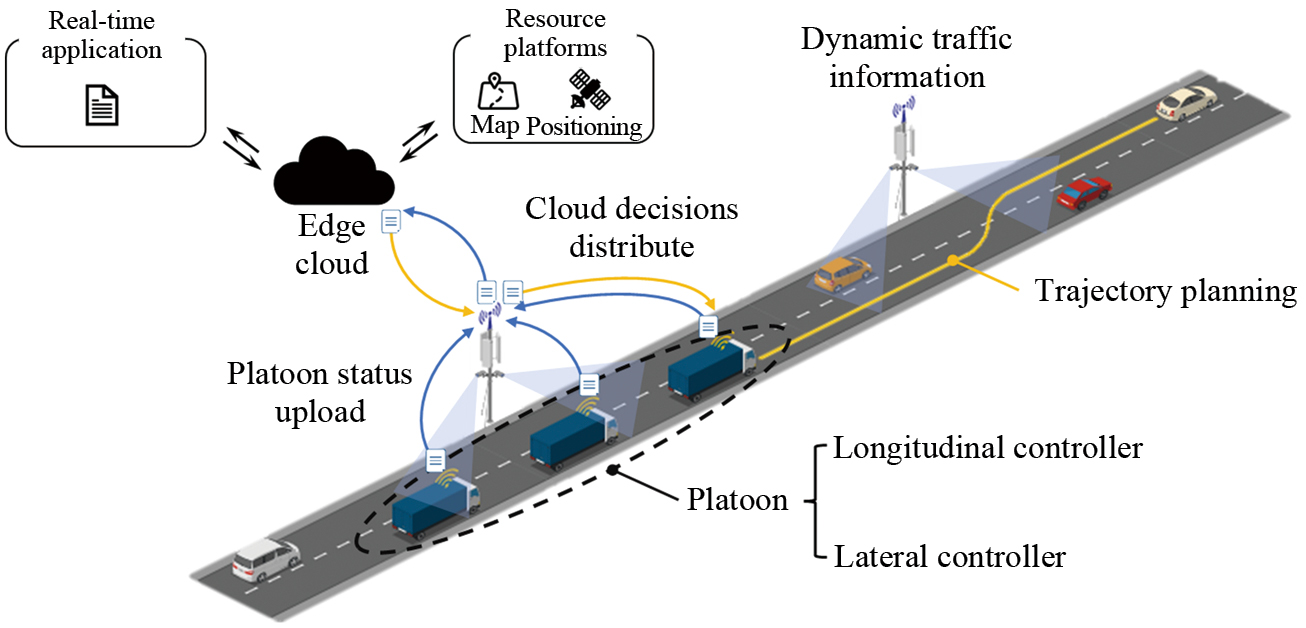
Based on the general architecture of CCS, the vehicle-cloud hierarchical control architecture is designed as shown in Fig. 2. The platoon travels on the highway and requests the platoon cooperative control service to the edge cloud. The edge cloud uses the communication network to obtain real-time status (e.g., position, speed, acceleration, gear, etc.) and vehicle parameter information (e.g., vehicle model) of the platoon vehicles and collects dynamic traffic information (e.g., location and speed of ambient vehicles) through the ICVs and roadside infrastructure. Vehicle parameters such as engine models are stored on the edge cloud and can be queried by the vehicle models uploaded by the platoon. The platoon collaborative control real-time application deployed in the cloud calculates the driving policy and dispatches the leader of the platoon. After receiving the cloud decision, the platoon analyzes whether the cloud decision is feasible according to the real-time traffic conditions, conducts trajectory planning and tracking control, and uploads the real-time vehicle status to form a rolling closed-loop control of the vehicle and cloud.
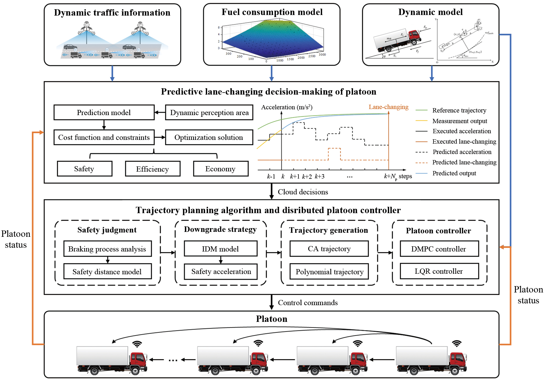
Based on the vehicle-cloud hierarchical control architecture, the CPPLC system is designed, including the PPLD as well as the trajectory planning algorithm and distributed platoon controller, as shown in Fig. 3. The PPLD algorithm is deployed in the cloud and mainly consists of dynamic perception area model, prediction model, cost function and hierarchical optimization solution, which takes dynamic traffic information, fuel consumption model, vehicle model and the status of platoon as inputs, and takes safety, efficiency and economy as optimization objectives to collaboratively optimize platoon longitudinal acceleration and lateral lane-changing decision-making. The trajectory planning algorithm and distributed platoon controller are deployed on the vehicle side, mainly including lane change safety judgment, degradation strategy, trajectory generation, and platoon controller, generating platoon driving trajectory and tracking control according to the decision issued from the cloud to ensure the safety of platoon driving.
The PPLD algorithm requires dynamic traffic information and fast computation. Using the digital mapping of traffic elements and efficient computation advantages of the CCS, it is arranged on the edge cloud to call the sensory information of roadside infrastructure and ICVs according to the vehicle positioning information for fast solution of the decision volume, which can realize the comprehensive improvement of the performance of platoon driving safety and efficiency.
The vehicle is a complex multi-degree-of-freedom dynamical system, and there are coupling effects between the longitudinal and lateral motions of the vehicle, and it is difficult to establish the vehicle dynamics model accurately. In this section, the longitudinal and lateral motions are decoupled, and the dynamics of the vehicle are modeled for few specific parameters by model simplification
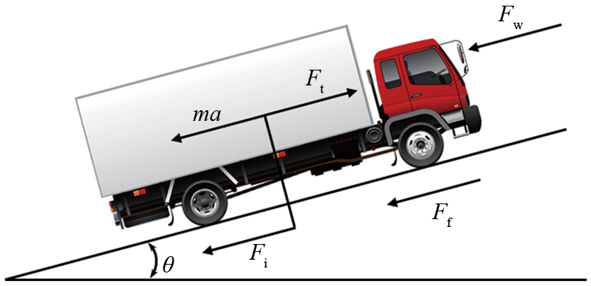
Consider the vehicle driving scenario as shown in Fig. 4, and analyze the forces of the vehicle(1)where m is the vehicle mass, a is the vehicle acceleration, Ft is the driving force, Ff is the rolling resistance, Fw is the air resistance, and Fi is the ramp resistance.
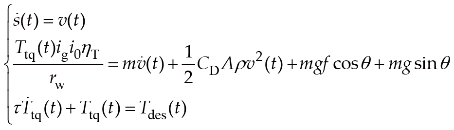
Expanding the drive and drag forces, Eq. (1) can be expressed by the following,(2)where Ttq is the engine torque, i0 is the main gear ratio, ig is the transmission ratio, ηT is the transmission efficiency, rw is the tire radius, CD is the air resistance coefficient, A is the windward area, ρ is the air density, v is the vehicle speed, g is the gravitational acceleration, f is the rolling resistance coefficient, and θ is the road slope angle.
Describe the longitudinal motion of the vehicle using a third-order nonlinear model:(3)where s is the longitudinal displacement of the vehicle, τ is the inertial hysteresis of the vehicle longitudinal dynamics, and is the desired torque.
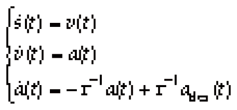
Based on the feedback linearization theory, the linearization of Eq. (3) leads to a third-order linear model of the vehicle [2]:(4)
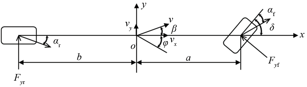
A linear two-degree-of-freedom model is used to describe the lateral dynamics of the vehicle [24], as shown in Fig. 5. In the figure, xoy is the body coordinate system, o is the center of mass of the vehicle, a and b are the lengths from the center of mass to the front and rear axes, respectively, vx and vy are the longitudinal and lateral vehicle speeds at the center of mass of the vehicle in the body coordinate system, δ is the front wheel rotation angle, φ is the transverse sway angle, β is the lateral deflection angle of the center of mass, αf and αr are the lateral deflection angles of the front and rear wheels, and Fyf and Fyr denote the lateral deflection forces of the front and rear wheels.
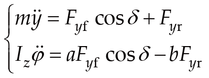
The differential equation is established by the lateral force balance and the torque balance around the z-axis:(5)
where Iz represents the rotational inertia of the center of mass around the z-axis.
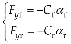
Fyf and Fyr can be expressed by the following equation:(6)
where Cf and Cr denote the lateral deflection stiffness of the front and rear wheels.
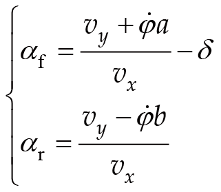
According to the geometric relationship between the vehicle coordinate system and the center of mass, αf and αr can be expressed by the following equation:(7)
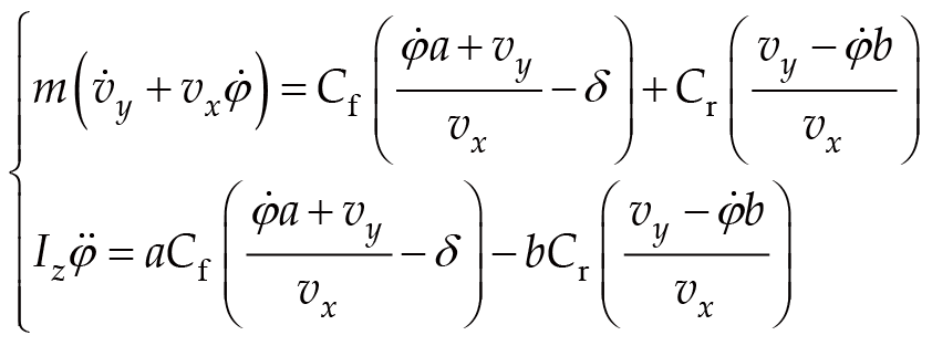
Combining Eqs. (5–7), the differential equation of lateral motion of the vehicle can be obtained:(8)
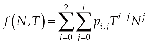
Based on the engine universal characteristic curve data of the vehicle, a polynomial curve fitting method is used to establish the fuel consumption model. The fuel consumption model is a quadratic polynomial function of engine speed and engine torque:(9)where, f denotes the fuel consumption per second, pi,j denotes the fitting factor, T denotes the engine torque, and N denotes the engine speed.
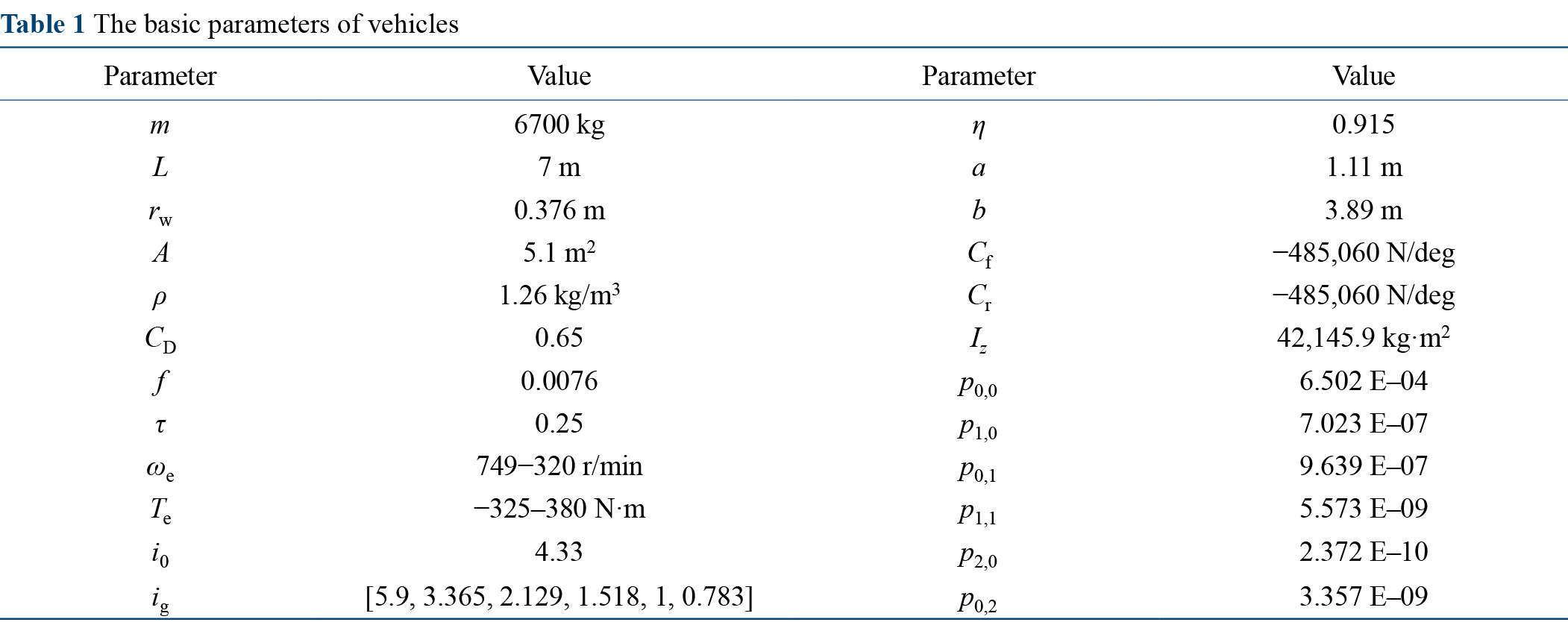
The basic parameters of the vehicles used in this paper are shown in Table 1.
This section designs the PPLD algorithm, firstly analyzes the platoon lane change strategy and clarifies the way of platoon lane change, then establishes the dynamic perception area model to find the environmental vehicles that may affect the platoon driving; then establishes the prediction model and constructs the multi-objective optimization problem, and finally designs the hierarchical solution strategy to collaboratively optimize the platoon longitudinal acceleration and lateral lane-changing decision-making.
The two main strategies on platoon lane change are synchronous and asynchronous [9], and a comparison of the two approaches is shown in Fig. 6.
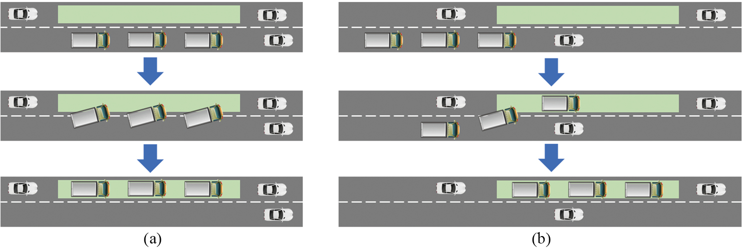
Synchronous lane change strategy requires all vehicles to change lanes at the same time, which is efficient, easy to control, and guarantees the integrity of the platoon, but is difficult to implement in dense traffic flows. Asynchronous lane change strategy requires vehicles in the platoon to change lanes sequentially, which allows the platoon to use smaller gaps during the lane change, but the lane change is inefficient and computationally intensive, and the platoon may be truncated by environmental vehicles during the lane change, requiring a more complex policy design to ensure the safety of the platoon.
Considering that the scenario is a highway, which is relatively simple compared with the urban road scenario, and the algorithm needs to ensure the integrity of the platoon, the synchronous lane change strategy is chosen. In addition, when using the synchronous lane change approach for lane-changing decision-making, the platoon can be regarded as a longer single vehicle, and the length of the platoon is determined by the leader and the tail vehicle of the platoon, which can reduce the complexity of the computational design of the decision algorithm.
The platoon driving on a two-lane highway, as shown in Fig. 7. The PPLD algorithm needs to determine the horizontal and lateral travel strategy of the platoon based on the real-time traffic conditions and future trends to improve the driving performance of the platoon.
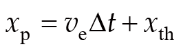
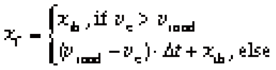
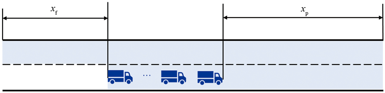
The PPLD algorithm requires dynamic traffic information, and considering too many environmental vehicles will lead to an increase in computing volume and a waste of computational resources while considering too few environmental vehicles will lead to a decrease in the value of computational results. Therefore, a dynamic perception area needs to be established to filter the environmental vehicles and find the environmental vehicles that may affect the platoon movement in the prediction horizon. As shown in Fig. 8, the blue area indicates the dynamic perception area. xp indicates the length of the forward perception area, and xf indicates the length of the rear perception area, and the values are given by Eqs. (10 and 11):(10)(11)where ve is the speed of the platoon at the beginning of the prediction, vroad is the road speed limit in the lane next to the platoon, Δt is the prediction duration, Δt=Np·ΔT, Np is the prediction horizon, ΔT is the time step size, and xth is a constant.
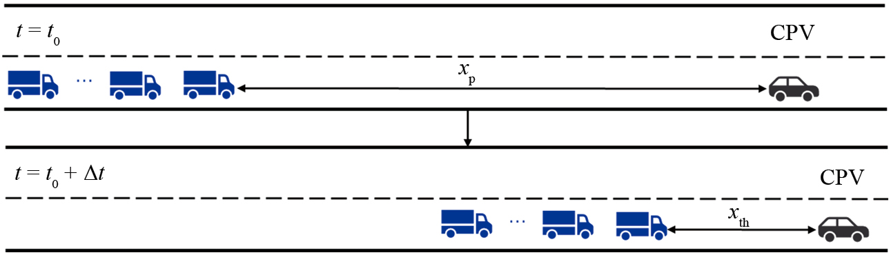
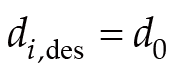
For the forward perception area, consider the scenario shown in Fig. 9. At t0, there exists a slow vehicle CPV in front of the platoon with initial distance xp. At t0+Δt, the platoon travels to the range xth behind the CPV, when the CPV affects the platoon travel. When the speed of CPV is 0, xp takes the maximum value, which indicates the limit distance ahead to be considered.
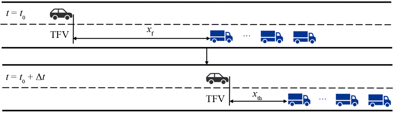
For the rear perception area, consider the scenario shown in Fig. 10. At t0, there exists a fast vehicle TFV behind the platoon side lane with initial distance xf. At t0+Δt, the TFV travels to the rear of the platoon within the range xth. At this time, the TFV affects the platoon's lane change. When the speed of platoon is higher than the speed limit of the side lane, TFV will not affect the platoon travel, and only the vehicles within range xth behind the platoon at the beginning of the prediction will be considered; when the speed of platoon is lower than the speed limit of the side lane and the speed of TFV is the road speed limit, xf takes the maximum value, indicating the limit range to be considered.
With the dynamic perception area, all environmental vehicles that may affect the platoon travel in the prediction horizon are filtered out and fed into the prediction model.
The prediction model uses historical information about the object and future control inputs to predict the future state of the object and to provide a priori information for subsequent optimization problems. In order to describe the problem more clearly, the following variables are defined for modeling a vehicle in discrete time that is in the dynamic perception area:
(m,n): the ID of the vehicle, m∈{L,R,E}, L denotes left lane, R denotes right lane, E denotes platoon vehicles, n∈{1,2,…}, the number increases sequentially from rear to front;
xm,n(k): the longitudinal position of vehicle (m,n) at step k;
vm,n(k): the longitudinal speed of vehicle (m,n) at step k;
δm,n(k): the lane of vehicle (m,n) at step k, δm,n(k)∈{0,1}, 0 denotes the right lane, 1 denotes the left lane;
Xm,n(k): the state of vehicle (m,n) at step k, ;
am,n(k): the longitudinal acceleration of vehicle (m,n) at step k;
λm,n(k): vehicle (m,n) changes lanes to the left at step k, λm,n(k)∈{0,1}, 0 and 1 indicate lane change and no lane change;
γm,n(k): vehicle (m,n) changes lanes to the right at step k, γm,n(k)∈{0,1}, 0 and 1 indicate lane change and no lane change;
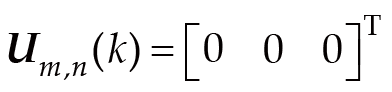
Um,n(k): the control command of vehicle (m,n) at step k,. Note that λm,n(k) and γm,n(k) cannot both be 1 at the same time.
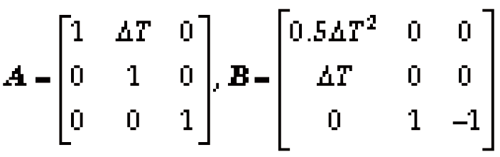
Define the state transfer equation of vehicle (m,n) as shown in the following:(12)where,
Considering that the application scenario of the algorithm is the highway, which is relatively simple compared to the urban road scenario, and the motion state of the vehicles on the road is relatively stable, the constant speed model is used to estimate the environmental vehicle state:(13)
In real traffic scenarios, vehicles may not follow the constant speed model and may change lanes due to factors such as different driving habits of drivers and interactions between vehicles, and the prediction model can be replaced using a more accurate model. In addition, within each discrete time step, the state information of the ambient vehicle is transmitted from the ICVs and the roadside infrastructure to the cloud control platform, which is used to correct the state of the ambient vehicle.
The cost function responds to the deviation degree of the actual state of the control object from the control objective, and multiple control objectives (e.g., economy, comfort, etc.) can be considered, and multiple control objectives are integrated to form a comprehensive performance index. The optimal control amount of the system is found by minimizing the cost function. For the PLCD algorithm, the following control objectives are mainly:
(1) collision risk: the platoon should minimize the risk of collision while driving;
(2) fuel economy: the platoon should work near the efficient operating zone of the engine to improve fuel economy;
(3) travel efficiency: the platoon should travel near the desired speed to improve travel efficiency;
(4) comfort: the platoon should accelerate and decelerate smoothly to improve driving comfort;
(5) desired lane: the platoon expects to drive in the right lane and should return to the desired lane as soon as possible after leaving the desired lane.
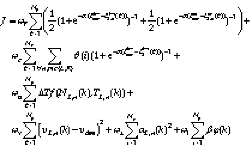
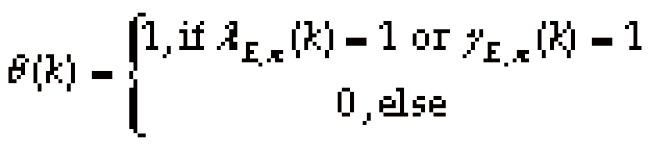
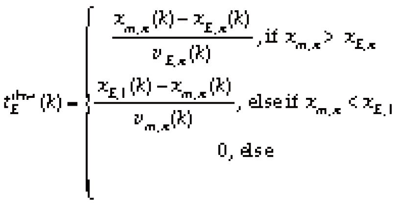
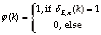
Based on the above control objectives, the following cost function was designed:(14)where,(15)(16)(17)where Np is the prediction horizon, Nc is the control horizon, ωf, ωc, ωo, ωv, ωa, ωl is the following weight, lane change weight, fuel consumption weight, speed weight, acceleration weight and lane weight respectively, and denote the safe headway time and safe collision time, and denote the actual headway time and actual collision time of the leader, θ(k) is used to determine whether the platoon is changing lanes, denotes the actual collision time between the platoon and the vehicle in the target lane, f(NE,i(k),TE,i(k)) denotes the fuel consumption per second of the platoon, NE,n(k) and TE,n(k) denote the engine speed and torque of the vehicle, vdes denotes the desired speed of the platoon, φ(k) is used to determine the lane of the platoon, α and β are constant.
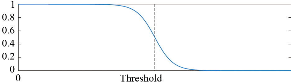
For the car-following cost and lane-changing cost, both take the form of Sigmoid functions, which are the main working area near the set threshold, as shown in Fig. 11. The car-following cost and the lane-changing cost can penalize the dangerous situation during the platoon driving and improve the safety of the queue driving.
Taking into account traffic rules, limitations of vehicle actuators and driving comfort, some constraints of the algorithm are defined:
(1) Speed constraint
The platoon must comply with the road traffic rules during travel, so the speed needs to be constrained, and denote the lower and upper bound of the road speed limit:(18)
(2) Actuator physical limitations
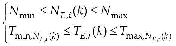
Due to the physical limitations of the actuator, the engine speed and torque must be within the actuating range of the actuator, Nmin and Nmax are the lower and upper bounds of engine speed, and are the lower and upper bounds of engine torque at engine speed NE,i(k):(19)
(3) Comfort requirements
A large acceleration change rate will make humans uncomfortable, so the acceleration change rate needs to be constrained, Δamin and Δamin are the lower and upper bounds of the acceleration change rate:(20)
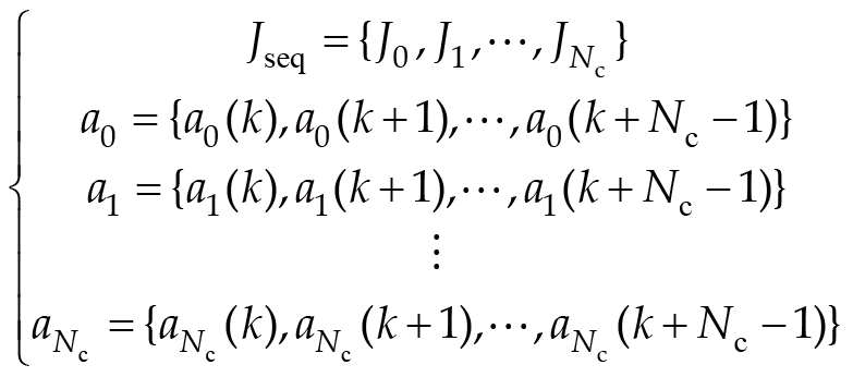
The quantity to be solved in the PPLD algorithm contains continuous acceleration and also 0−1 lane-changing decision-making, and the cost function and constraints contain nonlinear parts, so the problem is a mixed-integer nonlinear programming (MINLP) problem, and the solution of such problems is very difficult, and the problem needs to be simplified. Considering the high risk of platoon lane change, multiple lane-changing in a short time is not recommended. Therefore, it is assumed that the platoon makes at most one lane change in the control horizon. Based on this assumption, the problem can be decomposed into subproblems corresponding to no lane change, lane change at step 1, ..., and lane change at step Nc, respectively. For each subproblem, the quantity to be optimized is only the acceleration sequence, which can be solved by nonlinear programming, and the cost of each subproblem as well as the acceleration sequence is retained, as shown in the following equation:(21)
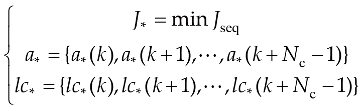
Next, the cost of Nc+1 subproblems is compared and the least costly subproblem is found, and the acceleration sequence and lane-changing decision-making sequence corresponding to this subproblem are the final optimization results:(22)
The overall flow of the algorithm (algorithm 1 PPLD) is as follows:
(1) initialize prediction horizon Np, control horizon Nc, time step size, state matrix ΔT, control matrix and other parameters;
(2) at step k, the dynamic perception area is calculated, the state of the ambient vehicle in the dynamic perception area range is obtained, and the future state of the ambient vehicle is predicted by the prediction model;
(3) decompose the optimization problem into Nc+1 subproblems, and for compute Jseq, compute Jseq and ai by min J;
(4) compare Jseq, find the smallest item J*, get the corresponding a* and lc*, and send the result to the vehicle end;
(5) set the current time to k+1 and repeat from step 2.
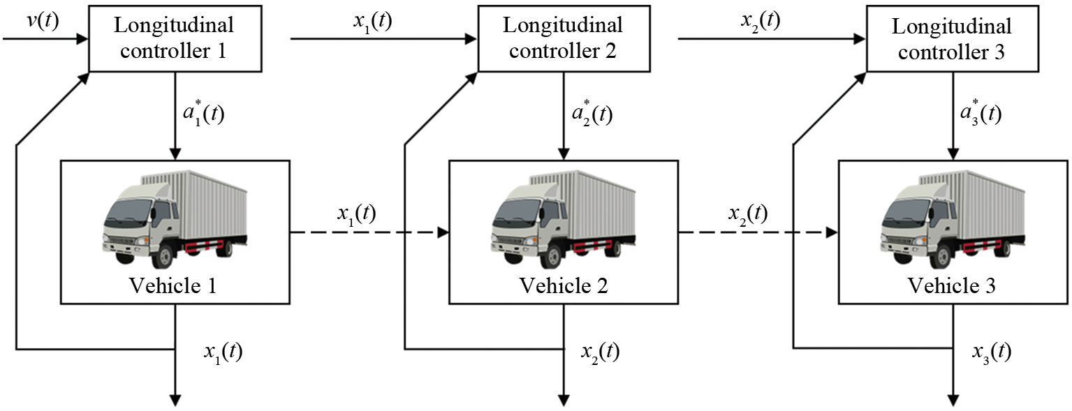
This section designs the trajectory planning algorithm and distributed platoon controller deployed on the vehicle side to complement the execution process of car-following and lane-changing. The trajectory planning algorithm is deployed on the leader vehicle, and the distributed platoon controller is deployed on all vehicles in the platoon. Since the synchronous platoon lane change method is selected, the paths of all vehicles are similar, and only the leader is required to perform trajectory planning and synchronize the planned paths to the following vehicle, which can calculate the driving path of the self-vehicle according to the desired vehicle spacing, and perform tracking control
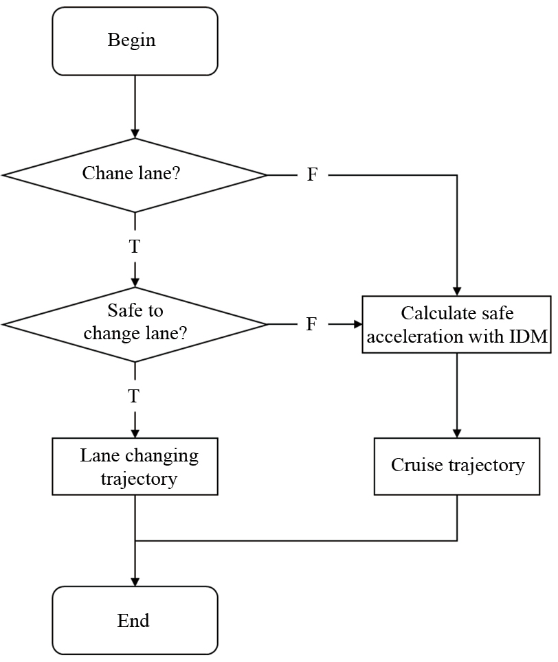
The process of trajectory planning is shown in Fig. 12, when the first value of lateral lane-changing decision-making sequence is lane change, it is necessary to judge the safety of lane change first, and carry out lane change trajectory planning when the judgment result is safe. When the judgment result is unsafe, the safe acceleration is calculated by IDM model and car-following trajectory planning is carried out; when the first value of lateral lane-changing decision-making sequence is no lane change, car-following trajectory planning is carried out directly.
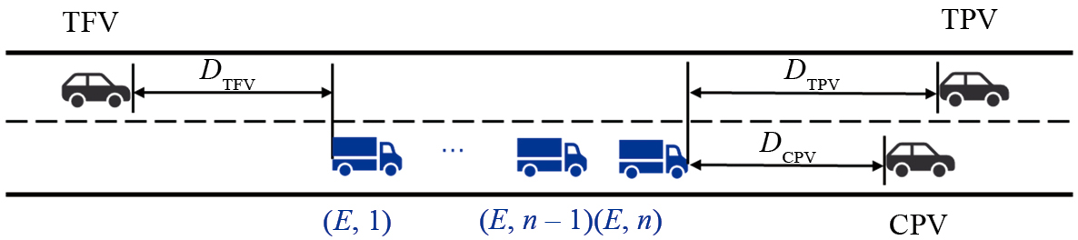
The platoon travels on the highway as shown in Fig. 13, using CPV to denote the vehicle in front of the current lane of the platoon, TPV to denote the vehicle in front of the target lane, and TFV to denote the vehicle behind the target lane, with DCPV and DTFV denoting the spacing between the leader vehicle (E,n) and the CPV and TPV, respectively, and DTFV denotes the spacing between the tail vehicle (E,1) and the TFV. The platoon needs to be collision-free and at a safe distance from the three environmental vehicles during the lane change.
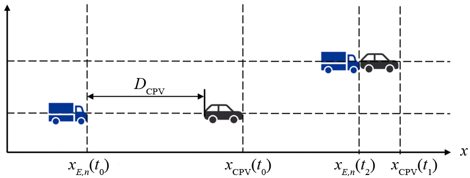
Take the leader vehicle (E,n) and CPV as an example to analyze the safety distance, as shown in Fig. 14. The CPV emergency brakes at t0 and stops at t1. The leader vehicle (E,n) brakes after a reaction time and stops at moment B. To ensure that no collisions occur, it is necessary to meet:(23)where xCPV(t1) and xE,n(t2) denote the position when CPV and (E,n) stop, and LCPV denotes the length of CPV.
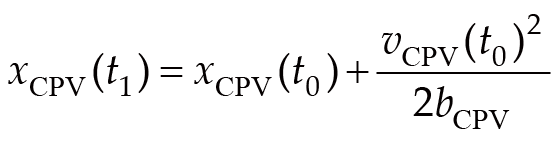
For CPV, the braking process can be considered as a constant deceleration process, A can be expressed by the following equation:(24)where bCPV denotes the maximum deceleration of CPV.
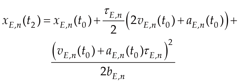
The (E,n) is ICV, the acceleration and speed of (E,n) are aE,n(t0) and vE,n(t0) at t0. Due to the delay in data processing and control system, (E,n) can not directly enter the braking state, it needs to pass time τE,n to enter the emergency braking state and travel at the maximum deceleration speed. (E,n) stops at t2 and the stop position of the (E,n) can be calculated as(25)
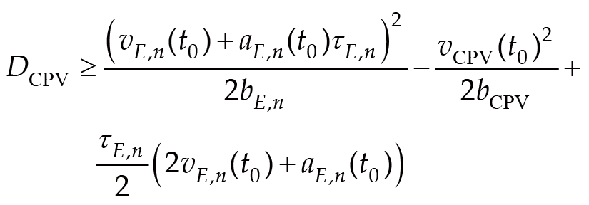
From Eqs. (23–25), the safety distance that needs to be satisfied by (E,n) and CPV can be calculated as(26)
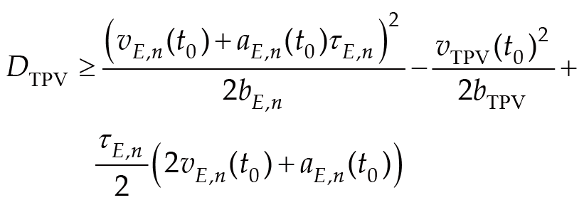
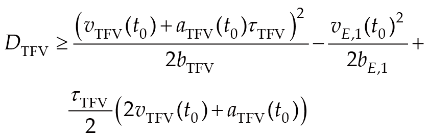
Similarly, it can be calculated that DTPV and DTFV need to satisfy the following conditions:(27)(28)where τTFV denotes the reaction time of the human driver.
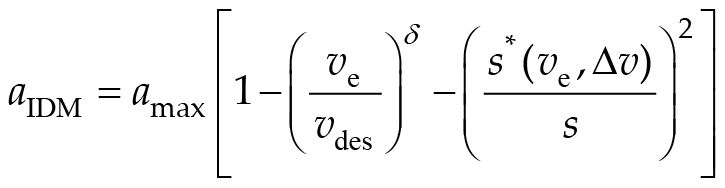
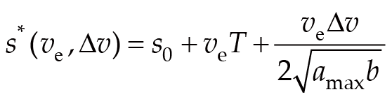
When the cloud decision is to change lanes, but the vehicle side judges that it is not safe to change lanes, a safety degradation strategy is designed to ensure the safety of platoon and wait for the next cycle of cloud commands. Safe acceleration is generated using the IDM model [25]:(29)(30)where aIDM denotes the acceleration of the target vehicle, amax denotes the maximum acceleration of the vehicle, ve denotes the speed of the target vehicle, vdes denotes the desired speed of the target vehicle, δ denotes the acceleration index, Δv denotes the speed difference between the target vehicle and the lead vehicle with the expression Δv=ve–vp, vp denotes the speed of the preceding vehicle, s*(ve, Δv) denotes the desired following distance of the target vehicle, s denotes the actual following distance between the target vehicle and the preceding vehicle with the expression s=xp–xe–lp, xp and xe denote the longitudinal position of the preceding vehicle and the target vehicle, respectively, lp denotes the body length of the lead vehicle, s0 denotes the stationary safety distance, T denotes the safe headway time distance, and b denotes the comfortable deceleration speed.
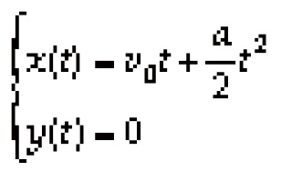
The car-following trajectory is generated based on the constant acceleration (CA) model(31)where x(t) and y(t) denote the longitudinal and lateral displacement of the vehicle, respectively, v0 denotes the longitudinal velocity of the vehicle at the beginning of the trajectory planning, and a denotes the desired acceleration.
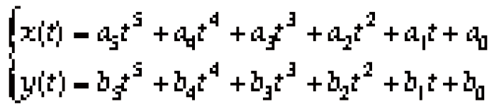
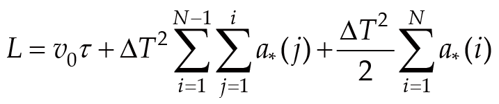
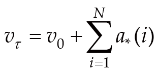
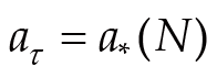
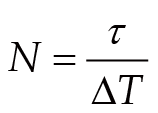
The lane-changing trajectory can be described by a fifth order polynomial curve(32)where v0 and a0 denote the longitudinal velocity and acceleration of the vehicle at the beginning of the trajectory planning, which can be measured by the on-board sensors, τ denotes the lane change duration, according to statistics, the vehicle lane change on the highway is generally completed within 5 s, a shorter lane change time can improve efficiency, but will lead to poor comfort, this paper chooses a fixed lane change duration (5 s), W denotes the lane width, L, vτ and aτ denote the longitudinal displacement, velocity and acceleration of the vehicle at the end of the lane change, which can be calculated by integrating the acceleration sequence sent down from the cloud in discrete time:(33)(34)(35)where, a* denotes the acceleration sequence sent down from the cloud, ΔT denotes the discrete step length of the PPLD algorithm, and N denotes the discrete time step of the lane change process, which can be expressed by the following equation:(36)
The lane-changing trajectory contains 12 unknown parameters, and 13 parameters of the start state, end state and lane change duration are known to uniquely determine the trajectory.
In this section, the platoon control problem is decomposed into platoon longitudinal control and lateral path tracking problem, and the longitudinal DMPC controller and the lateral LQR controller are designed respectively.
The DMPC controller is designed based on the PF communication topology. Defining the state of the ith vehicle in the platoon as xi =[sivi ai]T . Vehicle i receives the state information of the preceding vehicle through V2V technology, and the control input of the vehicle is obtained by solving the optimization problem based on the state of the self-vehicle as well as the state of the preceding vehicle, as shown in Fig. 15.
The longitudinal control objective is to follow the speed of the preceding vehicle and maintain the desired space from the preceding vehicle. Since the PPLD algorithm needs to consider the platoon length, the spacing strategy of CD is chosen in order to reduce the complexity of the decision algorithm:(37)
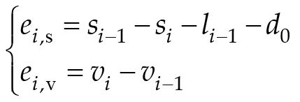
Define the spacing error and speed error of the ith vehicle as follows:(38)
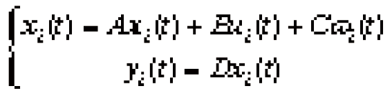
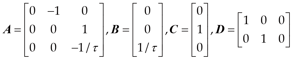
According to Eq. (4) and Eq. (43), the longitudinal error differential equation is defined:(39)where,where xi denotes the state vector, ui denotes the control input, ωi denotes the disturbance input, and yi denotes the system output.
The discrete state space model is created by discretizing Eq. (39):(40)where, , T denotes the discrete time step.
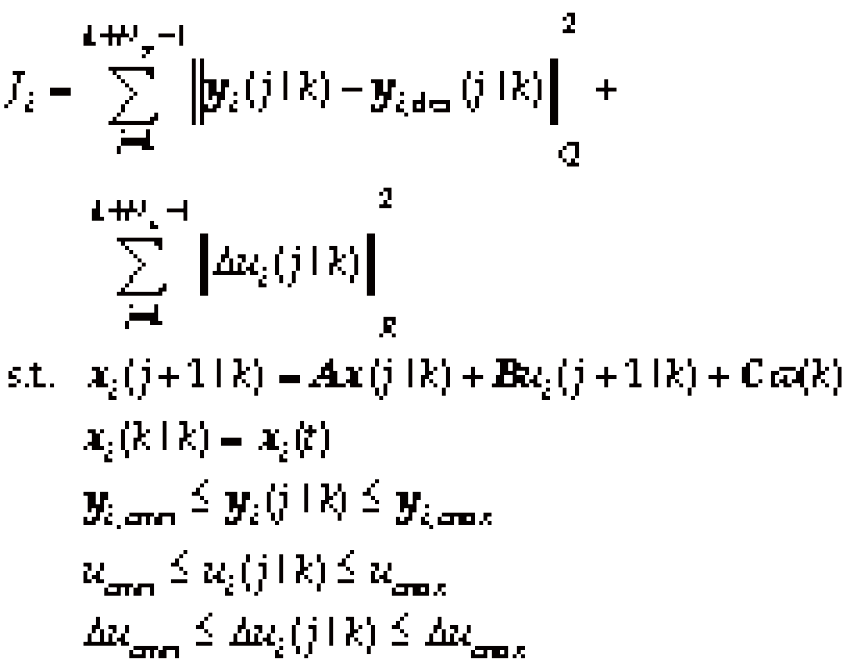
Define the control increment for vehicle i as , the system output as , and the desired output as . The goal of vehicle control is to reduce the spacing error and velocity error while avoiding large acceleration variations, which can be represented by the following cost function:(41)where Q and R denote the system error and control input weight matrix, yi,min and yi,max denote the minimum and maximum values of the system output, umin and umax denote the minimum and maximum values of the acceleration, Δumin and Δumax denote the minimum and maximum values of the rate of change of the acceleration.
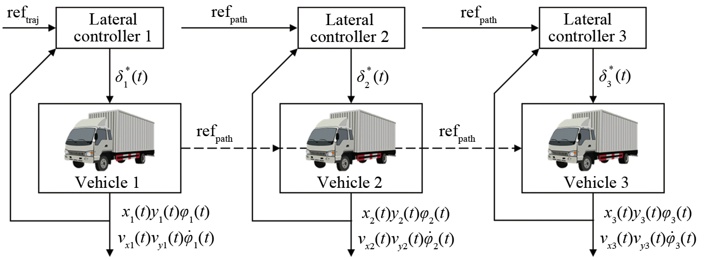
Based on the leader-following topology design lateral LQR controller, each vehicle in the platoon receives the path sent by the leader vehicle through V2V technology, calculates the path of the self-vehicle according to the spacing model, and combines the self-vehicle state to calculate the control input by solving the optimization problem to achieve the path tracking of the vehicle, as shown in Fig. 16.
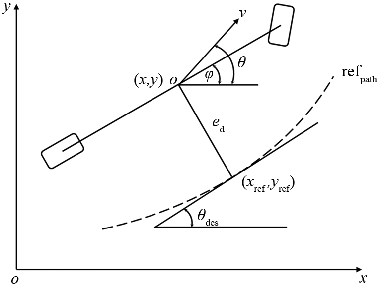
The vehicle is projected onto the reference path and the lateral path tracking error model is established, as shown in Fig. 17. In the figure, xoy denotes the geodesic coordinate system, (x,y) denotes the vehicle center of mass coordinates, φ denotes the yaw angle, θ denotes the heading angle, refpath denotes the reference path, (xref, yref )denotes the coordinates of the projection point, ed denotes the distance from the vehicle center of mass to the projection point, and θdes denotes the desired heading angle of the projection point.
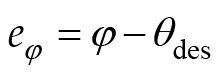
When the vehicle tracks the reference path, the spacing error is denoted using ed and the heading error eφ is defined as(42)
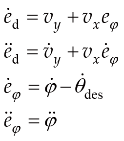
The derivatives of A and B can be expressed as:(43)
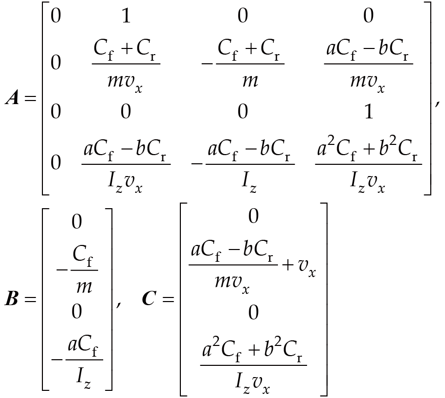
The lateral dynamics model (8) and the lateral error (47) can be rewritten in the form of a state space with state vector , control input u=δ and disturbance ω=θdes:(44)式中:
If the disturbance θdes in Eq. (48) is zero, then the lateral path tracking problem can be solved analytically using LQR. For a linear system, the control objective of LQR is to choose a suitable control law u*(t)=–Kx(t) such that the following performance indicator function takes the minimum value:(45)
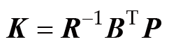
The feedback control law K can be given by the following equation:(46)where, K=[k1k2k3k4]T, P is the solution of Riccati equation ATP + PA – PBR−1BTP + Q =0.
Substituting the feedback control law u*(t) = –Kx(t) into Eq. (46) yields(47)
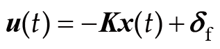
When , the system has a steady-state error due to the presence of θdes, x(t)≠0. To eliminate the steady-state error, it is necessary to introduce the feedforward control input δf, i.e:(48)
Substituting Eq. (48) into Eq. (46) and making , the feedforward control input δf that can eliminate the steady-state error of the spacing error ed is obtained:(49)
To verify the effectiveness of the proposed algorithm, a simulation environment is built based on Sumo, Matlab/Simulink and Trucksim. Sumo is used to generate microscopic traffic flow and simulate the dynamic traffic environment on the road, Trucksim is used to build the dynamics model of the platoon, and Matlab/Simulink is used to deploy the CPPLC algorithm.
In order to simulate the real situation of platoon driving and the effectiveness of the design algorithm in different scenarios, two simulation scenarios are designed.
As shown in Fig. 18, a platoon consisting of three vehicles travels on a two-lane highway, with the left side being the fast lane and equally spaced traffic on the road, and the right lane being the slow lane, with a slow vehicle traveling at a constant speed in front of the platoon, and the platoon will gradually be affected by the slow vehicle because the desired speed of the platoon is higher than the speed of the slow vehicle.
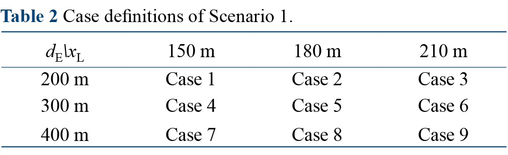
In order to verify whether the algorithm can work under different initial conditions, nine cases of examples were designed, as shown in Table 2.
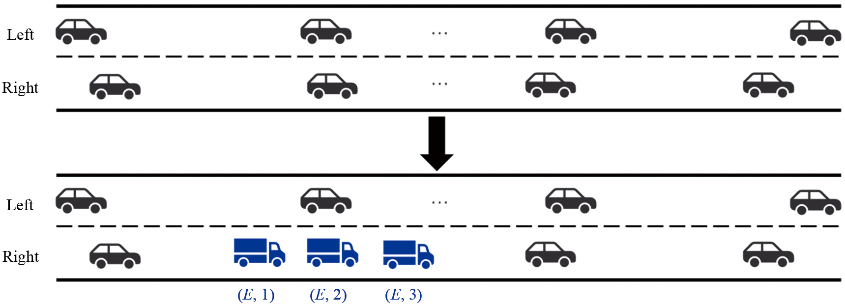
As shown in Fig. 19, there is a steady flow of traffic on a two-lane highway in both the left and right lanes. At the beginning of the simulation a platoon of three vehicles is substituted for an ambient vehicle in the right lane, and the desired speed of the platoon is higher than the desired speed of the traffic flow on the right side and lower than the desired speed of the traffic flow on the left side.
In order to verify the effectiveness of the algorithm under different traffic flows, five cases of examples under different traffic flows are designed, as shown in Table 3.
All ambient vehicles on the road are generated by Sumo and the motion state is updated using the IDM model and the LC2013 model [26]. Two controllers were evaluated
(1) CPPLC: The method can collaboratively optimize the longitudinal acceleration and lateral lane change timing of the platoon to improve the platoon driving performance.
(2) Baseline: Microscopic driving models, using the IDM model and MOBIL model [27] to generate longitudinal acceleration and lateral lane change decisions.
The following performance measurements are adopted.
(1) Safety: Inverse time-to-collision model (TTCi) [28]. When TTCi≤0, it means that there is no collision risk, and when TTCi>0, the collision risk increases with the increase of TTCi value. In the collision warning system, the common warning threshold of TTC is 2.5–4 s [29], which corresponds to a TTCi of 0.25–0.4 s−1, and the threshold of 0.2 s−1 is chosen in this paper. The leader vehicle of the platoon (denoted as PL) and the follower of the tail vehicle of the platoon (denoted as PF) are used as target vehicles to record the TTCi during the simulation. If TTCi is less than the set threshold, the platon driving strategy is considered safe, otherwise it is considered dangerous.
(2) Economy: Fuel consumption per 100 km.
(3) Efficiency: Average speed.
The main weighting coefficients of the CPPLC algorithm are shown in the Table 4.
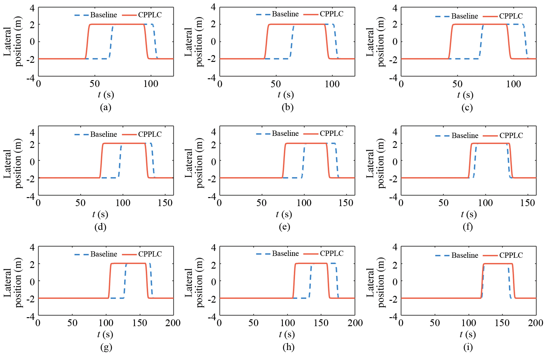
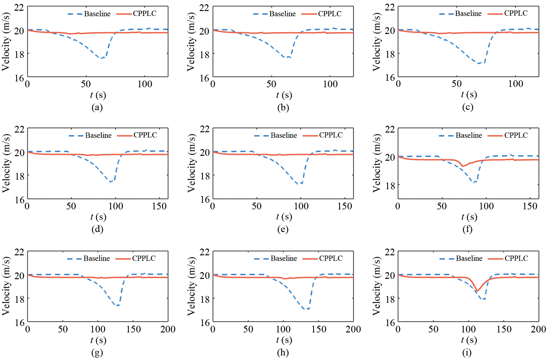
Figures 20 and 21 show the lateral position and speed curves of the leader vehicle respectively, from which it can be seen that the lane change moment of CPPLC is earlier than that of Baseline, and the speed is less influenced by the slow vehicle. the lane change model of Baseline is a real-time decision, in each discrete time to determine whether the current safety criterion and the incentive criterion of the MOBIL model are satisfied at the same time, and if they are satisfied, then execute lane change. Due to the influence of the slow vehicle, Baseline has a significant speed decay before finding the time to change lanes. In contrast, CPPLC is equipped with environmental vehicle state and trend prediction model, which can find the optimal lane change timing and the corresponding acceleration sequence in advance by solving the optimization problem, making the platoon less affected by environmental vehicles and the speed decay when encountering the slow vehicle is significantly smaller than Baseline.
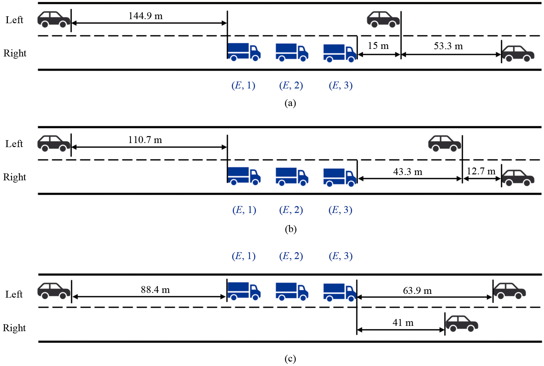
The first lane change of CPPLC is analyzed by Case 6. CPPLC finds the least costly subproblem by solving the optimization problem containing multiple objectives based on the prediction results and executes the corresponding acceleration sequence and lane-changing decision-making sequence. In 0–74 s, the cost of the no lane change subproblem is the lowest, and the decision of CPPLC is no lane change. As the distance between the platoon and the slow vehicle gets closer, the cost of the no-lane change subproblem gradually increases, and in 67–74 s, the acceleration sequence shows a large deceleration and the platoon speed produces a significant decay. When t=74 s, the subproblem cost corresponding to the first step lane change is the lowest, CPPLC finds the lane change timing, and the acceleration sequence becomes positive, at which time the relative position of the platoon and the surrounding vehicles is shown in Fig. 22 (a), and the target gap of the platoon lane change is the left rear gap. As time passes, the least costly subproblem continues to move forward. When t=79 s, the step 1 lane change subproblem has the lowest cost and the platoon performs a lane change, at which point the relative position of the platoon to the surrounding vehicles is shown in Fig. 22 (b). When t=84 s, the platoon has finished changing lanes, at this time the relative positions of the queue and the surrounding vehicles are shown in Fig. 22(c).
From Fig. 20(f), we can find that the platoon has passed the slow vehicle sometime before the end of the simulation, and the platoon is driving freely, but the speed of CPPLC is slightly lower than Baseline. this is due to the existence of fuel consumption cost in the cost function of CPPLC, and the fuel economy of the vehicle will be improved when the vehicle speed is lower, and the two optimization objectives of expected vehicle speed and economy are in conflict, so the speed of CPPLC will be slightly lower than that of Baseline.
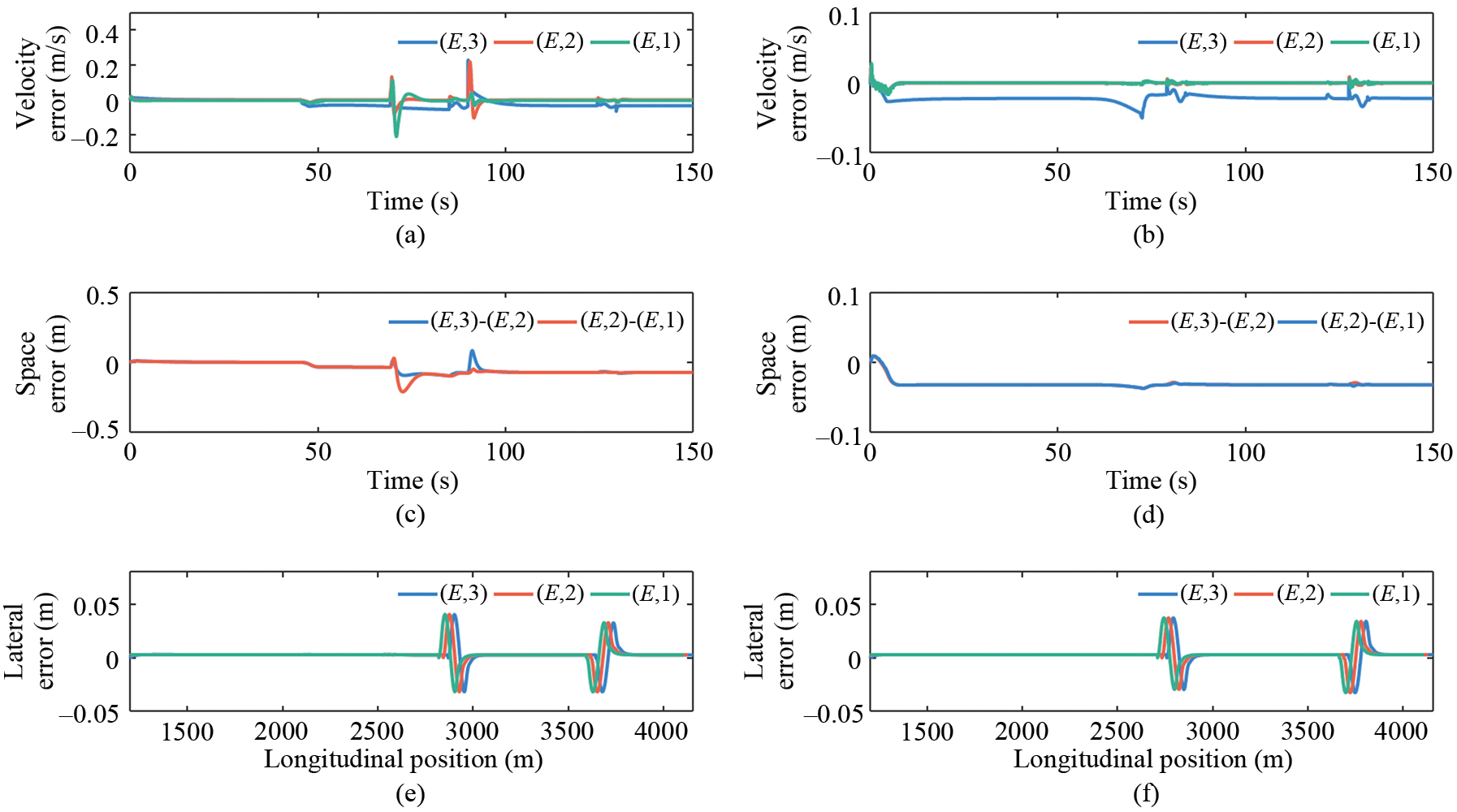
The tracking control effect of Case 6 is shown in Fig. 23. From figures (a)–(d), it can be seen that the leader vehicle can track the planned speed better, and the other vehicles in the platoon can track the speed of the previous vehicle better and keep a stable space from the previous vehicle. The speed error is between –0.2–0.3 m/s2 and the space error is between –0.3–0.1 m. From Fig. 23 (c), it can be seen that the algorithm can achieve synchronous platoon lane change and better tracking of the path with lateral error between –0.05–0.05 m. In addition, it can be found from the figure that the tracking control of CPPLC is better than Baseline. The reason for the analysis is that the speed fluctuation of CPPLC is smaller than that of Baseline, so the error caused by the speed fluctuation will be smaller.
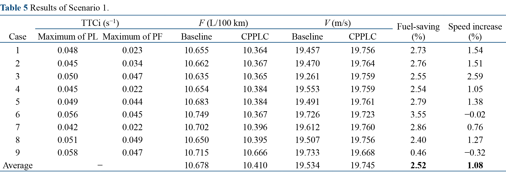
Table 5 gives the results of simulation Scenario 1. In terms of safety, the maximum value of TTCi for PL and PF in all cases is less than the threshold, indicating that CPPLC can ensure driving safety. In terms of fuel economy, the fuel consumption per 100 km (F) of CPPLC is lower than that of Baseline in all cases, with an average fuel saving rate of 2.52%. In terms of efficiency, Baseline performs better in Case 6 and Case 9, with CPPLC performing better in the other seven cases, with an average speed increase of 1.08% compared to Baseline.
Figures 24 and 25 show the lateral position and velocity curves of the leader vehicle. As can be seen from the figures, the CPPLC algorithm works equally well in the traffic flow, where the platoon lane change moment is earlier than Baseline and the number and magnitude of speed decay is smaller. Since the ambient vehicles in the right lane are traveling at a speed lower than the desired speed of the platoon, Baseline generates significant speed decay before finding the lane change moment, while CPPLC can find the acceleration and lane change moment earlier by solving the optimization problem because it has the ambient vehicle state prediction model, making the platoon less affected by the ambient vehicles.
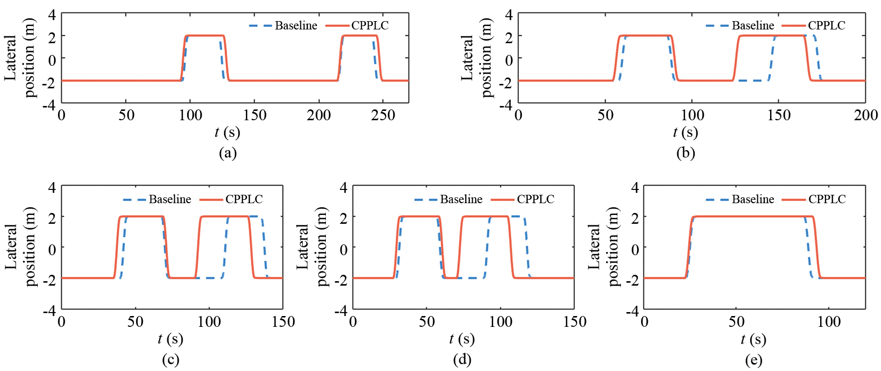
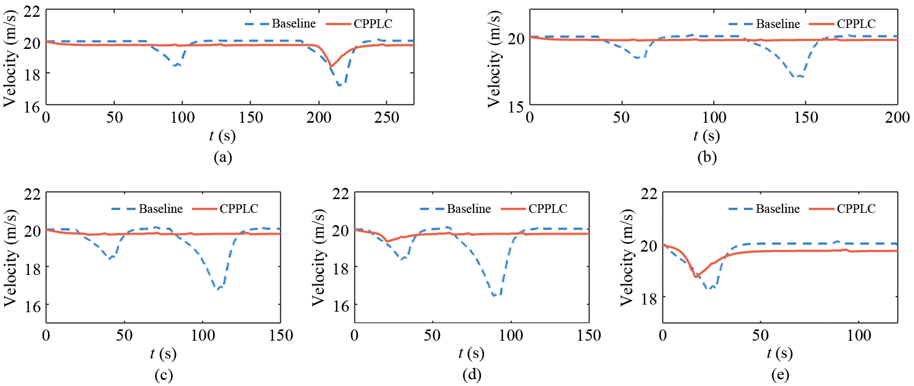
The maximum flow is set to 600 veh/h in simulation Scenario 2, as the control object is a platoon and synchronous lane-changing is adopted. Only when there is a large gap, the platoon has enough space and motivation for lane-changing. As seen in Fig. 25 (e), when the traffic flow reaches 600 veh/h, whether it is Baseline or CPPLC, after the platoon changes to the left lane, the platoon no longer has the maneuvering space to rejoin the right lane due to the smaller gap and slower speed of the right lane, and will keep driving in the left lane until the right lane is free of ambient traffic. It can be expected that the results will be similar to Case 5 when the traffic flow continues to increase until the platoon no longer changes lanes and loses its simulation value.
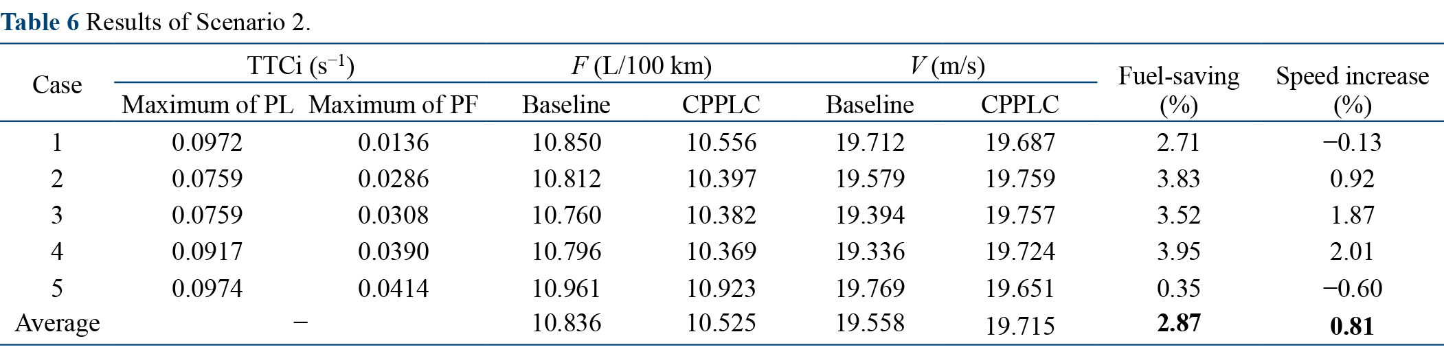
The results of simulation Scenario 2 are given in Table 6. In terms of safety, the maximum values of TTCi for PL and PF in all cases are less than the set threshold, indicating that CPPLC can ensure driving safety in all cases. In terms of fuel economy, the fuel consumption per 100 km of CPPLC is lower than that of Baseline in all cases, with an average fuel saving rate of 2.87%. In terms of efficiency, the optimization space of CPPLC is relatively small in Case 1 and Case 5 due to low or high traffic flow, so the performance of CPPLC is basically consistent with Baseline. In other cases, CPPLC is better than Baseline, and overall, CPPLC has an average speed increase of 0.81% compared to Baseline.
In the context of vehicle-road-cloud integration, this paper proposes a predictive lane-changing control scheme for platoons. The cloud-based algorithm considers both the car-following and lane-changing strategies of the platoon, which can extend the dimensionality of the search and improve the optimality of the optimization results compared with the existing PCC. At the same time, the use of predictive information enables the lane-changing strategy to take into account the future long-term expected benefits of the platoon driving, which helps the platoon obtain longer-term returns. A trajectory planning algorithm and a distributed platoon controller are deployed on the vehicle side in conjunction with the cloud-based algorithm to complement the execution process of car-following and lane-changing. Finally, a simulation platform is built and simulation experiments are conducted according to the scheme proposed in this paper. The experimental results show that the algorithm proposed in this paper can be adapted to various traffic scenarios and outperforms the comparison algorithms in terms of efficiency and economy while ensuring safety.
While the research in this paper is encouraging, it is worth noting that the scenarios in this paper still have limitations. We have designed the special scenarios described in this paper to demonstrate the advantages of the algorithm here. In future research, more traffic flows with stochasticity should be designed to verify the generalizability of the algorithm.
This work was supported by the National Key R & D Program of China (No. 2021YFB2501000) and the Joint R & D Project with Weichai Power Co., Ltd.
S. Wei, Y. Zou, X. Zhang, T. Zhang, and X. Li, "An integrated longitudinal and lateral vehicle following control system with radar and vehicle-to-vehicle communication," IEEE Transactions on Vehicular Technology, vol. 68, no. 2, pp. 1116–1127, 2019.
Y. Zheng, S. E. Li, J. Wang, D. Cao, and K. Li, "Stability and scalability of homogeneous vehicular platoon: Study on the influence of information flow topologies," IEEE Transactions on intelligent transportation systems, vol. 17, no. 1, pp. 14–26, 2015.
S. Feng, Y. Zhang, S. E. Li, Z. Cao, H. X. Liu, and L. Li, "String stability for vehicular platoon control: Definitions and analysis methods," Annual Reviews in Control, vol. 47, pp. 81–97, 2019.
B. Gao, K. Wan, Q. Chen, Z. Wang, R. Li, Y. Jiang, R. Mei, Y. Luo, and K. Li, "A review and outlook on predictive cruise control of vehicles and typical applications under cloud control system," Machine Intelligence Research, vol. 20, pp. 614–639, 2023.
F. Lattemann, K. Neiss, S. Terwen, and T. Connolly, "The predictive cruise control – A system to reduce fuel consumption of heavy duty trucks," SAE transactions, vol. 113, pp. 139–146, 2004.
H. Chu, L. Guo, B. Gao, H. Chen, N. Bian, and J. Zhou, "Predictive cruise control using high-definition map and real vehicle implementation," IEEE Transactions on Vehicular Technology, vol. 67, no. 12, pp. 11377–11389, 2018.
V. Turri, B. Besselink, and K. H. Johansson, "Cooperative look-ahead control for fuel-efficient and safe heavy-duty vehicle platooning," IEEE Transactions on Control Systems Technology, vol. 25, no. 1, pp. 12–28, 2016.
C. Zhai, F. Luo, Y. Liu, and Z. Chen, "Ecological cooperative look-ahead control for automated vehicles travelling on freeways with varying slopes," IEEE Transactions on Vehicular Technology, vol. 68, no. 2, pp. 1208–1221, 2018.
H. Wang, X. Li, X. Zhang, J. Hu, X. R. Yan, and Y. W. Feng, "Cut through traffic like a snake: Cooperative adaptive cruise control with successive platoon lane-change capability," Journal of Intelligent Transportation Systems, vol. 28, pp. 141–162, 2023.
A. Vahidi and A. Sciarretta, "Energy saving potentials of connected and automated vehicles," Transportation Research Part C: Emerging Technologies, vol. 95, pp. 822–843, 2018.
P. G. Gipps, "A model for the structure of lane-changing decision," Transportation Research Part B Methodological, vol. 20, no. 5, pp. 403–414, 1986.
G. Xiong, Z. Kang, H. Li, W. L. Song, Y. Y. Jin, and J. W. Gong, "Decision-making of lane change behavior based on RCS for automated vehicles in the real environment,"2018 IEEE Intelligent Vehicles Symposium (IV), IEEE, 2018, pp. 1400–1405.
J. Nilsson, J. Silvlin, M. Brannstrom, E. Coelingh, and J. Fredriksson, "If, when, and how to perform lane change maneuvers on highways," IEEE Intelligent Transportation Systems Magazine, vol. 8, no. 4, pp. 68–78, 2016.
Z. Feng, W. J. Song, M. Y. Fu, Y. Yang, and M. L. Wang, "Decision-making and path planning for highway autonomous driving based on spatio-temporal lane-change gaps," IEEE Systems Journal, vol. 16, no. 2, pp. 3249–3259, 2021.
W. Wang, T. Qie, C. Yang, W. Liu, and K. Huang, "An intelligent lane-changing behavior prediction and decision-making strategy for an autonomous vehicle," IEEE Transactions on Industrial Electronics, vol. 69, no. 3, pp. 2927–2937, 2021.
S. Li, C. Wei, and Y. Wang, "Combining decision making and trajectory planning for lane changing using deep reinforcement learning," IEEE Transactions on Intelligent Transportation Systems, vol. 23, no. 9, pp. 16110–16136, 2022.
Q. Zhang, R. Langari, H. E. Tseng, D. Filev, S. Szwabowski, and S. Coskun, "A game theoretic model predictive controller with aggressiveness estimation for mandatory lane change," IEEE Transactions on Intelligent Vehicles, vol. 5, no. 1, pp. 75–89, 2020.
G. Wang, J. Hu, Z. Li, and L. Li, "Harmonious lane changing via deep reinforcement learning," IEEE Transactions on Intelligent Transportation Systems, vol. 99, pp. 1–9, 2021.
K. Li, J. Li, X. Chang, B. Gao, and J. Pan, "Principle and typical application of cloud control system for intelligent networked vehicles," Journal of Automotive Safety and Energy Conservation, vol. 11, no. 3, pp. 261–275, 2020.
K. Li, X. Chang, J. Li, Q. Xu, B. Gao, and J. Pan, "Cloud control system for intelligent and connected vehicles and its application," Automotive Engineering, vol. 42, no. 12, pp. 1595–1605, 2020.
F. Zhao, J. Wang, T. Zhang, L. Wang, and D. Li, "Model predictive control method for vehicle platoon under cloud control scenes," Automotive Engineering, vol. 44, no. 2, pp. 179–189, 2022.
S. Li, K. Wan, B. Gao, R. Li, Y. Wang, and K. Li, "Predictive cruise control for heavy trucks based on slope information under cloud control system," Journal of Systems Engineering and Electronics, vol. 33, no. 4, pp. 812–826, 2022.
B. Gao, Q. Chen, Y. Liu, K. Wan, K. Li, "Predictive cruise control under cloud control system for urban bus considering queue dissipation time," IEEE Transactions on Intelligent Vehicles, vol. 8, no. 4, pp. 2639–2649, 2023.
S. Xu and H. Peng, "Design, analysis, and experiments of preview path tracking control for autonomous vehicles," IEEE Transactions on Intelligent Transportation Systems, vol. 21, no. 1, pp. 48–58, 2019.
M. Treiber, A. Hennecke, and D. Helbing, "Congested traffic states in empirical observations and microscopic simulations," Physical Review E, vol. 62, no. 2, p. 1805, 2000.
P. A. Lopez, M. Behrisch, L. Bieker-Walz, J. Erdma, Y.-P. Flötteöd, R. Hilbrich, L. Lücken, J. Rummel, P. Wagner, and E. WieBner, "Microscopic traffic simulation using SUMO,"2018 21st International Conference on Intelligent Transportation Systems (ITSC), Hawaii, USA, 2018, pp. 2575–2582.
A. Kesting, M. Treiber, and D. Helbing, "General lane-changing model mobil for car following models," Transportation Research Record Journal of the Transportation Research Board, vol. 1999. pp. 86–94, 2007.
R. J. Kiefer, D. J. LeBlanc, and C. A. Flannagan, "Developing an inverse time-to-collision crash alert timing approach based on drivers’ last-second braking and steering judgments," Accident Analysis & Prevention, vol. 37, no. 2, pp. 295–303, 2005.
 Top
Top